Statistics with R, Notes
Foreword
Output options: the ‘tango’ syntax and the ‘readable’ theme.
Codes and snippets.
Descriptive Statistics
Extract basic, exploratory statistics from datasets with apply, summary, fivenum, describe, and stat.desc.
# dataset
head ( longley , 3 )
## GNP.deflator GNP Unemployed Armed.Forces Population Year Employed
## 1947 83.0 234.289 235.6 159.0 107.608 1947 60.323
## 1948 88.5 259.426 232.5 145.6 108.632 1948 61.122
## 1949 88.2 258.054 368.2 161.6 109.773 1949 60.171
# apply a function
# excluding missing values
sapply ( longley , mean , na.rm = TRUE )
## GNP.deflator GNP Unemployed Armed.Forces Population
## 101.6813 387.6984 319.3313 260.6687 117.4240
## Year Employed
## 1954.5000 65.3170
# mean, median, 25th and 75th quartiles, min, max
summary ( longley )
1
2
3
4
5
6
7
8
9
10
11
12
13
14 ## GNP.deflator GNP Unemployed Armed.Forces
## Min. : 83.00 Min. :234.3 Min. :187.0 Min. :145.6
## 1st Qu.: 94.53 1st Qu.:317.9 1st Qu.:234.8 1st Qu.:229.8
## Median :100.60 Median :381.4 Median :314.4 Median :271.8
## Mean :101.68 Mean :387.7 Mean :319.3 Mean :260.7
## 3rd Qu.:111.25 3rd Qu.:454.1 3rd Qu.:384.2 3rd Qu.:306.1
## Max. :116.90 Max. :554.9 Max. :480.6 Max. :359.4
## Population Year Employed
## Min. :107.6 Min. :1947 Min. :60.17
## 1st Qu.:111.8 1st Qu.:1951 1st Qu.:62.71
## Median :116.8 Median :1954 Median :65.50
## Mean :117.4 Mean :1954 Mean :65.32
## 3rd Qu.:122.3 3rd Qu.:1958 3rd Qu.:68.29
## Max. :130.1 Max. :1962 Max. :70.55
# Tukey min, lower-hinge, median, upper-hinge, max
fivenum ( longley $ GNP )
## [1] 234.289 306.787 381.427 463.625 554.894
# n, nmiss, unique, mean, 5, 10, 25, 50, 75, 90, 95th percentiles
# 5 lowest and 5 highest scores
library ( Hmisc )
describe ( longley )
1
2
3
4
5
6
7
8
9
10
11
12
13
14
15
16
17
18
19
20
21
22
23
24
25
26
27
28
29
30
31
32
33
34
35
36
37
38
39
40
41
42
43
44
45
46
47
48
49
50
51
52
53
54
55
56
57
58
59
60
61
62
63
64
65
66
67
68
69
70
71
72
73
74
75
76
77
78
79
80
81
82
83
84
85
86
87
88
89
90
91
92
93
94
95
96
97
98
99
100
101
102 ## longley
##
## 7 Variables 16 Observations
## ---------------------------------------------------------------------------
## GNP.deflator
## n missing distinct Info Mean Gmd .05 .10
## 16 0 16 1 101.7 12.74 86.90 88.35
## .25 .50 .75 .90 .95
## 94.53 100.60 111.25 114.95 116.00
##
## Value 83.0 88.2 88.5 89.5 96.2 98.1 99.0 100.0 101.2 104.6
## Frequency 1 1 1 1 1 1 1 1 1 1
## Proportion 0.062 0.062 0.062 0.062 0.062 0.062 0.062 0.062 0.062 0.062
##
## Value 108.4 110.8 112.6 114.2 115.7 116.9
## Frequency 1 1 1 1 1 1
## Proportion 0.062 0.062 0.062 0.062 0.062 0.062
## ---------------------------------------------------------------------------
## GNP
## n missing distinct Info Mean Gmd .05 .10
## 16 0 16 1 387.7 117.8 252.1 258.7
## .25 .50 .75 .90 .95
## 317.9 381.4 454.1 510.4 527.4
##
## Value 234.289 258.054 259.426 284.599 328.975 346.999 363.112 365.385
## Frequency 1 1 1 1 1 1 1 1
## Proportion 0.062 0.062 0.062 0.062 0.062 0.062 0.062 0.062
##
## Value 397.469 419.180 442.769 444.546 482.704 502.601 518.173 554.894
## Frequency 1 1 1 1 1 1 1 1
## Proportion 0.062 0.062 0.062 0.062 0.062 0.062 0.062 0.062
## ---------------------------------------------------------------------------
## Unemployed
## n missing distinct Info Mean Gmd .05 .10
## 16 0 16 1 319.3 110.1 191.6 201.6
## .25 .50 .75 .90 .95
## 234.8 314.4 384.2 434.4 471.2
##
## Value 187.0 193.2 209.9 232.5 235.6 282.2 290.4 293.6 335.1 357.8
## Frequency 1 1 1 1 1 1 1 1 1 1
## Proportion 0.062 0.062 0.062 0.062 0.062 0.062 0.062 0.062 0.062 0.062
##
## Value 368.2 381.3 393.1 400.7 468.1 480.6
## Frequency 1 1 1 1 1 1
## Proportion 0.062 0.062 0.062 0.062 0.062 0.062
## ---------------------------------------------------------------------------
## Armed.Forces
## n missing distinct Info Mean Gmd .05 .10
## 16 0 16 1 260.7 79.85 155.7 160.3
## .25 .50 .75 .90 .95
## 229.8 271.8 306.1 344.9 355.9
##
## Value 145.6 159.0 161.6 165.0 251.4 255.2 257.2 263.7 279.8 282.7
## Frequency 1 1 1 1 1 1 1 1 1 1
## Proportion 0.062 0.062 0.062 0.062 0.062 0.062 0.062 0.062 0.062 0.062
##
## Value 285.7 304.8 309.9 335.0 354.7 359.4
## Frequency 1 1 1 1 1 1
## Proportion 0.062 0.062 0.062 0.062 0.062 0.062
## ---------------------------------------------------------------------------
## Population
## n missing distinct Info Mean Gmd .05 .10
## 16 0 16 1 117.4 8.229 108.4 109.2
## .25 .50 .75 .90 .95
## 111.8 116.8 122.3 126.6 128.4
##
## Value 107.608 108.632 109.773 110.929 112.075 113.270 115.094 116.219
## Frequency 1 1 1 1 1 1 1 1
## Proportion 0.062 0.062 0.062 0.062 0.062 0.062 0.062 0.062
##
## Value 117.388 118.734 120.445 121.950 123.366 125.368 127.852 130.081
## Frequency 1 1 1 1 1 1 1 1
## Proportion 0.062 0.062 0.062 0.062 0.062 0.062 0.062 0.062
## ---------------------------------------------------------------------------
## Year
## n missing distinct Info Mean Gmd .05 .10
## 16 0 16 1 1954 5.667 1948 1948
## .25 .50 .75 .90 .95
## 1951 1954 1958 1960 1961
##
## Value 1947 1948 1949 1950 1951 1952 1953 1954 1955 1956
## Frequency 1 1 1 1 1 1 1 1 1 1
## Proportion 0.062 0.062 0.062 0.062 0.062 0.062 0.062 0.062 0.062 0.062
##
## Value 1957 1958 1959 1960 1961 1962
## Frequency 1 1 1 1 1 1
## Proportion 0.062 0.062 0.062 0.062 0.062 0.062
## ---------------------------------------------------------------------------
## Employed
## n missing distinct Info Mean Gmd .05 .10
## 16 0 16 1 65.32 4.153 60.28 60.72
## .25 .50 .75 .90 .95
## 62.71 65.50 68.29 69.45 69.81
##
## Value 60.171 60.323 61.122 61.187 63.221 63.639 63.761 64.989 66.019
## Frequency 1 1 1 1 1 1 1 1 1
## Proportion 0.062 0.062 0.062 0.062 0.062 0.062 0.062 0.062 0.062
##
## Value 66.513 67.857 68.169 68.655 69.331 69.564 70.551
## Frequency 1 1 1 1 1 1 1
## Proportion 0.062 0.062 0.062 0.062 0.062 0.062 0.062
## ---------------------------------------------------------------------------
# nbr.val, nbr.null, nbr.na, min max, range, sum,
# median, mean, SE.mean, CI.mean, var, std.dev, coef.var
library ( pastecs )
stat.desc ( longley )
 1
 2
 3
 4
 5
 6
 7
 8
 9
10
11
12
13
14
15
16
17
18
19
20
21
22
23
24
25
26
27
28
29
30 ## GNP.deflator GNP Unemployed Armed.Forces
## nbr.val 16.0000000 16.0000000 16.0000000 16.0000000
## nbr.null 0.0000000 0.0000000 0.0000000 0.0000000
## nbr.na 0.0000000 0.0000000 0.0000000 0.0000000
## min 83.0000000 234.2890000 187.0000000 145.6000000
## max 116.9000000 554.8940000 480.6000000 359.4000000
## range 33.9000000 320.6050000 293.6000000 213.8000000
## sum 1626.9000000 6203.1750000 5109.3000000 4170.7000000
## median 100.6000000 381.4270000 314.3500000 271.7500000
## mean 101.6812500 387.6984375 319.3312500 260.6687500
## SE.mean 2.6978884 24.8487344 23.3616062 17.3979901
## CI.mean.0.95 5.7504129 52.9638237 49.7940849 37.0829381
## var 116.4576250 9879.3536593 8732.2342917 4843.0409583
## std.dev 10.7915534 99.3949378 93.4464247 69.5919604
## coef.var 0.1061312 0.2563718 0.2926316 0.2669747
## Population Year Employed
## nbr.val 1.600000e+01 1.600000e+01 1.600000e+01
## nbr.null 0.000000e+00 0.000000e+00 0.000000e+00
## nbr.na 0.000000e+00 0.000000e+00 0.000000e+00
## min 1.076080e+02 1.947000e+03 6.017100e+01
## max 1.300810e+02 1.962000e+03 7.055100e+01
## range 2.247300e+01 1.500000e+01 1.038000e+01
## sum 1.878784e+03 3.127200e+04 1.045072e+03
## median 1.168035e+02 1.954500e+03 6.550400e+01
## mean 1.174240e+02 1.954500e+03 6.531700e+01
## SE.mean 1.739025e+00 1.190238e+00 8.779921e-01
## CI.mean.0.95 3.706645e+00 2.536932e+00 1.871396e+00
## var 4.838735e+01 2.266667e+01 1.233392e+01
## std.dev 6.956102e+00 4.760952e+00 3.511968e+00
## coef.var 5.923918e-02 2.435893e-03 5.376806e-02
# item name, item number, nvalid, mean, sd,
# median, mad, min, max, skew, kurtosis, se
library ( psych )
describe ( longley )
1
2
3
4
5
6
7
8
9
10
11
12
13
14
15
16 ## vars n mean sd median trimmed mad min max
## GNP.deflator 1 16 101.68 10.79 100.60 101.93 15.79 83.00 116.90
## GNP 2 16 387.70 99.39 381.43 386.71 118.57 234.29 554.89
## Unemployed 3 16 319.33 93.45 314.35 317.26 116.75 187.00 480.60
## Armed.Forces 4 16 260.67 69.59 271.75 261.84 52.78 145.60 359.40
## Population 5 16 117.42 6.96 116.80 117.22 8.17 107.61 130.08
## Year 6 16 1954.50 4.76 1954.50 1954.50 5.93 1947.00 1962.00
## Employed 7 16 65.32 3.51 65.50 65.31 4.31 60.17 70.55
## range skew kurtosis se
## GNP.deflator 33.90 -0.13 -1.40 2.70
## GNP 320.61 0.02 -1.35 24.85
## Unemployed 293.60 0.14 -1.30 23.36
## Armed.Forces 213.80 -0.37 -1.20 17.40
## Population 22.47 0.26 -1.27 1.74
## Year 15.00 0.00 -1.43 1.19
## Employed 10.38 -0.09 -1.55 0.88
# with
with ( longley , median ( GNP ))
# vs.
median ( longley $ GNP )
Group data
# dataset
head ( mtcars , 3 )
## mpg cyl disp hp drat wt qsec vs am gear carb
## Mazda RX4 21.0 6 160 110 3.90 2.620 16.46 0 1 4 4
## Mazda RX4 Wag 21.0 6 160 110 3.90 2.875 17.02 0 1 4 4
## Datsun 710 22.8 4 108 93 3.85 2.320 18.61 1 1 4 1
# variable grouped by one factor to show a function
by ( mtcars $ mpg , mtcars $ cyl , FUN = function ( x ) { c ( m = mean ( x ), s = sd ( x )) })
## mtcars$cyl: 4
## m s
## 26 . 663636 4 . 509828
## --------------------------------------------------------
## mtcars$cyl: 6
## m s
## 19 . 742857 1 . 453567
## --------------------------------------------------------
## mtcars$cyl: 8
## m s
## 15 . 100000 2 . 560048
# description statistics by group
library ( psych )
describeBy ( mtcars , group = mtcars $ am )
 1
 2
 3
 4
 5
 6
 7
 8
 9
10
11
12
13
14
15
16
17
18
19
20
21
22
23
24
25
26
27
28
29
30
31
32
33
34
35
36
37
38
39
40
41
42
43
44
45
46
47
48
49
50
51
52
53 ##
## Descriptive statistics by group
## group: 0
## vars n mean sd median trimmed mad min max range
## mpg 1 19 17.15 3.83 17.30 17.12 3.11 10.40 24.40 14.00
## cyl 2 19 6.95 1.54 8.00 7.06 0.00 4.00 8.00 4.00
## disp 3 19 290.38 110.17 275.80 289.71 124.83 120.10 472.00 351.90
## hp 4 19 160.26 53.91 175.00 161.06 77.10 62.00 245.00 183.00
## drat 5 19 3.29 0.39 3.15 3.28 0.22 2.76 3.92 1.16
## wt 6 19 3.77 0.78 3.52 3.75 0.45 2.46 5.42 2.96
## qsec 7 19 18.18 1.75 17.82 18.07 1.19 15.41 22.90 7.49
## vs 8 19 0.37 0.50 0.00 0.35 0.00 0.00 1.00 1.00
## am 9 19 0.00 0.00 0.00 0.00 0.00 0.00 0.00 0.00
## gear 10 19 3.21 0.42 3.00 3.18 0.00 3.00 4.00 1.00
## carb 11 19 2.74 1.15 3.00 2.76 1.48 1.00 4.00 3.00
## skew kurtosis se
## mpg 0.01 -0.80 0.88
## cyl -0.95 -0.74 0.35
## disp 0.05 -1.26 25.28
## hp -0.01 -1.21 12.37
## drat 0.50 -1.30 0.09
## wt 0.98 0.14 0.18
## qsec 0.85 0.55 0.40
## vs 0.50 -1.84 0.11
## am NaN NaN 0.00
## gear 1.31 -0.29 0.10
## carb -0.14 -1.57 0.26
## --------------------------------------------------------
## group: 1
## vars n mean sd median trimmed mad min max range skew
## mpg 1 13 24.39 6.17 22.80 24.38 6.67 15.00 33.90 18.90 0.05
## cyl 2 13 5.08 1.55 4.00 4.91 0.00 4.00 8.00 4.00 0.87
## disp 3 13 143.53 87.20 120.30 131.25 58.86 71.10 351.00 279.90 1.33
## hp 4 13 126.85 84.06 109.00 114.73 63.75 52.00 335.00 283.00 1.36
## drat 5 13 4.05 0.36 4.08 4.02 0.27 3.54 4.93 1.39 0.79
## wt 6 13 2.41 0.62 2.32 2.39 0.68 1.51 3.57 2.06 0.21
## qsec 7 13 17.36 1.79 17.02 17.39 2.34 14.50 19.90 5.40 -0.23
## vs 8 13 0.54 0.52 1.00 0.55 0.00 0.00 1.00 1.00 -0.14
## am 9 13 1.00 0.00 1.00 1.00 0.00 1.00 1.00 0.00 NaN
## gear 10 13 4.38 0.51 4.00 4.36 0.00 4.00 5.00 1.00 0.42
## carb 11 13 2.92 2.18 2.00 2.64 1.48 1.00 8.00 7.00 0.98
## kurtosis se
## mpg -1.46 1.71
## cyl -0.90 0.43
## disp 0.40 24.19
## hp 0.56 23.31
## drat 0.21 0.10
## wt -1.17 0.17
## qsec -1.42 0.50
## vs -2.13 0.14
## am NaN 0.00
## gear -1.96 0.14
## carb -0.21 0.60
# description statistics by group
library ( doBy )
summaryBy ( mpg + wt ~ cyl + vs , data = mtcars ,
FUN = function ( x ) { c ( m = mean ( x ), s = sd ( x )) } )
## cyl vs mpg.m mpg.s wt.m wt.s
## 1 4 0 26.00000 NA 2.140000 NA
## 2 4 1 26.73000 4.7481107 2.300300 0.5982073
## 3 6 0 20.56667 0.7505553 2.755000 0.1281601
## 4 6 1 19.12500 1.6317169 3.388750 0.1162164
## 5 8 0 15.10000 2.5600481 3.999214 0.7594047
Frequency Tables, CrossTables, and Independence
Create frequency and contingency tables from categorical variables. Perform tests of independence, measures of association, and graphically display results.
2D frequency tables
mytable <- table(A, B) where A are rows, B are columns.
# dataset
mytable <- matrix ( c ( 1 , 2 , 3 , 4 ), nrow = 2 )
mytable
## [,1] [,2]
## [1,] 1 3
## [2,] 2 4
# A frequencies (summed over columns = 1)
margin.table ( mytable , 1 )
# B frequencies (summed over rows = 2)
margin.table ( mytable , 2 )
# A/(A + B)
# cell percentages
prop.table ( mytable )
## [,1] [,2]
## [1,] 0.1 0.3
## [2,] 0.2 0.4
# row percentages
prop.table ( mytable , 1 )
## [,1] [,2]
## [1,] 0.2500000 0.7500000
## [2,] 0.3333333 0.6666667
# column percentages
prop.table ( mytable , 2 )
## [,1] [,2]
## [1,] 0.3333333 0.4285714
## [2,] 0.6666667 0.5714286
3D frequency tables
## Grouped Data: uptake ~ conc | Plant
## Plant Type Treatment conc uptake
## 1 Qn1 Quebec nonchilled 95 16.0
## 2 Qn1 Quebec nonchilled 175 30.4
## 3 Qn1 Quebec nonchilled 250 34.8
A <- as.numeric ( CO2 [, 'Plant' ])
B <- CO2 [, 'conc' ]
C <- CO2 [, 'uptake' ]
mytable <- table ( A , B , C )
# several arrays (3D)
dim ( mytable ) # the printout is immense
# folded table (2D)
dim ( ftable ( mytable )) # the printout is immense
# 3-Way frequency Table
mytable <- xtabs ( ~ A + B + C , data = mytable , na.action = na.omit )
dim ( ftable ( mytable )) # the printout is immense
CrossTable
A <- as.numeric ( CO2 [ 1 : 8 , 'Plant' ])
A
## [1] 95 175 250 350 500 675 1000 95
# 2-way cross tabulation
library ( gmodels )
CrossTable ( A , B ) # mydata$myrowvar x mydata$mycolvar
 1
 2
 3
 4
 5
 6
 7
 8
 9
10
11
12
13
14
15
16
17
18
19
20
21
22
23
24
25
26
27
28
29
30
31
32
33
34
35 ##
##
## Cell Contents
## |-------------------------|
## | N |
## | Chi-square contribution |
## | N / Row Total |
## | N / Col Total |
## | N / Table Total |
## |-------------------------|
##
##
## Total Observations in Table: 8
##
##
## | B
## A | 95 | 175 | 250 | 350 | 500 | 675 | 1000 | Row Total |
## -------------|-----------|-----------|-----------|-----------|-----------|-----------|-----------|-----------|
## 1 | 1 | 1 | 1 | 1 | 1 | 1 | 1 | 7 |
## | 0.321 | 0.018 | 0.018 | 0.018 | 0.018 | 0.018 | 0.018 | |
## | 0.143 | 0.143 | 0.143 | 0.143 | 0.143 | 0.143 | 0.143 | 0.875 |
## | 0.500 | 1.000 | 1.000 | 1.000 | 1.000 | 1.000 | 1.000 | |
## | 0.125 | 0.125 | 0.125 | 0.125 | 0.125 | 0.125 | 0.125 | |
## -------------|-----------|-----------|-----------|-----------|-----------|-----------|-----------|-----------|
## 2 | 1 | 0 | 0 | 0 | 0 | 0 | 0 | 1 |
## | 2.250 | 0.125 | 0.125 | 0.125 | 0.125 | 0.125 | 0.125 | |
## | 1.000 | 0.000 | 0.000 | 0.000 | 0.000 | 0.000 | 0.000 | 0.125 |
## | 0.500 | 0.000 | 0.000 | 0.000 | 0.000 | 0.000 | 0.000 | |
## | 0.125 | 0.000 | 0.000 | 0.000 | 0.000 | 0.000 | 0.000 | |
## -------------|-----------|-----------|-----------|-----------|-----------|-----------|-----------|-----------|
## Column Total | 2 | 1 | 1 | 1 | 1 | 1 | 1 | 8 |
## | 0.250 | 0.125 | 0.125 | 0.125 | 0.125 | 0.125 | 0.125 | |
## -------------|-----------|-----------|-----------|-----------|-----------|-----------|-----------|-----------|
##
##
Tests of independence
There are more tests of independence in section 10, Resampling Statistics.
# dataset, a contingency table
colors
## fair.hair red.hair medium.hair dark.hair black.hair
## blue eyes 326 38 241 110 3
## light eyes 688 116 584 188 4
## medium eyes 343 84 909 412 26
## dark eyes 98 48 403 681 85
# chi-square test on 2-way tables
# test independence of the row and column variables, p-value is calculated from the asymptotic chi-squared distribution of the test statistic
chisq.test ( colors )
##
## Pearson's Chi-squared test
##
## data: colors
## X-squared = 1240, df = 12, p-value < 2.2e-16
# dataset, a contingency table in 2x2 matrix form
TeaTasting <-
matrix ( c ( 3 , 1 , 1 , 3 ),
nrow = 2 ,
dimnames = list ( Guess = c ( "Milk" , "Tea" ),
Truth = c ( "Milk" , "Tea" )))
TeaTasting
## Truth
## Guess Milk Tea
## Milk 3 1
## Tea 1 3
# Fisher exact test
fisher.test ( TeaTasting , alternative = "greater" )
##
## Fisher ' s Exact Test for Count Data
##
## data : TeaTasting
## p - value = 0 .2429
## alternative hypothesis : true odds ratio is greater than 1
## 95 percent confidence interval :
## 0 .3135693 Inf
## sample estimates :
## odds ratio
## 6 .408309
# 3D contingency table, where the last dimension refers to the strata
Rabbits <-
array ( c ( 0 , 0 , 6 , 5 ,
3 , 0 , 3 , 6 ,
6 , 2 , 0 , 4 ,
5 , 6 , 1 , 0 ,
2 , 5 , 0 , 0 ),
dim = c ( 2 , 2 , 5 ),
dimnames = list (
Delay = c ( "None" , "1.5h" ),
Response = c ( "Cured" , "Died" ),
Penicillin.Level = c ( "1/8" , "1/4" , "1/2" , "1" , "4" )))
Rabbits
1
2
3
4
5
6
7
8
9
10
11
12
13
14
15
16
17
18
19
20
21
22
23
24
25
26
27
28
29
30
31
32
33
34 ## , , Penicillin.Level = 1/8
##
## Response
## Delay Cured Died
## None 0 6
## 1.5h 0 5
##
## , , Penicillin.Level = 1/4
##
## Response
## Delay Cured Died
## None 3 3
## 1.5h 0 6
##
## , , Penicillin.Level = 1/2
##
## Response
## Delay Cured Died
## None 6 0
## 1.5h 2 4
##
## , , Penicillin.Level = 1
##
## Response
## Delay Cured Died
## None 5 1
## 1.5h 6 0
##
## , , Penicillin.Level = 4
##
## Response
## Delay Cured Died
## None 2 0
## 1.5h 5 0
# Mantel-Haenszel test / Cochran-Mantel-Haenszel chi-squared test, hypothesis that two nominal variables are conditionally independent in each stratum, assuming that there is no three-way interaction.
mantelhaen.test ( Rabbits )
##
## Mantel-Haenszel chi-squared test with continuity correction
##
## data: Rabbits
## Mantel-Haenszel X-squared = 3.9286, df = 1, p-value = 0.04747
## alternative hypothesis: true common odds ratio is not equal to 1
## 95 percent confidence interval:
## 1.026713 47.725133
## sample estimates:
## common odds ratio
## 7
# dataset
# 3-way contingency table based on variables A, B, and C
A <- CO2 [, 'Plant' ]
B <- CO2 [, 'conc' ]
C <- CO2 [, 'uptake' ]
mytable <- xtabs ( ~ A + B + C ) # a 3D array
# loglinear Models
# mutual independence: A, B, and C are pairwise independent
library ( MASS )
loglm ( ~ A + B + C , mytable )
## Call:
## loglm(formula = ~A + B + C, data = mytable)
##
## Statistics:
## X^2 df P(> X^2)
## Likelihood Ratio 720.1035 6291 1.0000000
## Pearson 6300.0000 6291 0.4656775
# conditional independence: A is independent of B, given C
loglm ( ~ A + B + C + A * C + B * C , mytable )
## Call:
## loglm(formula = ~A + B + C + A * C + B * C, data = mytable)
##
## Statistics:
## X^2 df P(> X^2)
## Likelihood Ratio 12.13685 5016 1
## Pearson NaN 5016 NaN
# no three-way interaction
loglm ( ~ A + B + C + A * B + A * C + B * C , mytable )
## Call:
## loglm(formula = ~A + B + C + A * B + A * C + B * C, data = mytable)
##
## Statistics:
## X^2 df P(> X^2)
## Likelihood Ratio 1.038376 4950 1
## Pearson NaN 4950 NaN
Measures of association
Association between two nominal variables, giving a value between 0 and +1 (inclusive). It is based on Pearson’s chi-squared statistic.
## 'data.frame': 84 obs. of 5 variables:
## $ ID : int 57 46 77 17 36 23 75 39 33 55 ...
## $ Treatment: Factor w/ 2 levels "Placebo","Treated": 2 2 2 2 2 2 2 2 2 2 ...
## $ Sex : Factor w/ 2 levels "Female","Male": 2 2 2 2 2 2 2 2 2 2 ...
## $ Age : int 27 29 30 32 46 58 59 59 63 63 ...
## $ Improved : Ord.factor w/ 3 levels "None"<"Some"<..: 2 1 1 3 3 3 1 3 1 1 ...
tab <- xtabs ( ~ Improved + Treatment , data = Arthritis )
tab
## Treatment
## Improved Placebo Treated
## None 29 13
## Some 7 7
## Marked 7 21
1
2
3
4
5
6
7
8
9
10
11
12
13 ##
## Call : xtabs ( formula = ~ Improved + Treatment , data = Arthritis )
## Number of cases in table : 84
## Number of factors : 2
## Test for independence of all factors :
## Chisq = 13 .055 , df = 2 , p - value = 0 .001463
## X ^ 2 df P ( > X ^ 2 )
## Likelihood Ratio 13 .530 2 0 .0011536
## Pearson 13 .055 2 0 .0014626
##
## Phi - Coefficient : NA
## Contingency Coeff .: 0 .367
## Cramer ' s V : 0.394
# phi coefficient, contingency coefficient, and Cramér's V for an 2D table
library ( vcd )
assocstats ( tab )
## X^2 df P(> X^2)
## Likelihood Ratio 13.530 2 0.0011536
## Pearson 13.055 2 0.0014626
##
## Phi-Coefficient : NA
## Contingency Coeff.: 0.367
## Cramer's V : 0.394
## Truth
## Guess Milk Tea
## Milk 3 1
## Tea 1 3
# Cohen's kappa and weighted kappa for a confusion matrix
library ( vcd )
kappa ( TeaTasting )
Correlations
# dataset
head ( mtcars , 3 )
##                mpg cyl disp  hp drat    wt  qsec vs am gear carb
## Mazda RX4     21.0   6  160 110 3.90 2.620 16.46  0  1    4    4
## Mazda RX4 Wag 21.0   6  160 110 3.90 2.875 17.02  0  1    4    4
## Datsun 710    22.8   4  108  93 3.85 2.320 18.61  1  1    4    1
# correlations/covariances among numeric variables in
# a data frame
cor ( mtcars , use = "complete.obs" , method = "kendall" ) # method = "pearson", "spearman" or "kendall"
 1
 2
 3
 4
 5
 6
 7
 8
 9
10
11
12
13
14
15
16
17
18
19
20
21
22
23
24 ## mpg cyl disp hp drat wt
## mpg 1.0000000 -0.7953134 -0.7681311 -0.7428125 0.46454879 -0.7278321
## cyl -0.7953134 1.0000000 0.8144263 0.7851865 -0.55131785 0.7282611
## disp -0.7681311 0.8144263 1.0000000 0.6659987 -0.49898277 0.7433824
## hp -0.7428125 0.7851865 0.6659987 1.0000000 -0.38262689 0.6113081
## drat 0.4645488 -0.5513178 -0.4989828 -0.3826269 1.00000000 -0.5471495
## wt -0.7278321 0.7282611 0.7433824 0.6113081 -0.54714953 1.0000000
## qsec 0.3153652 -0.4489698 -0.3008155 -0.4729061 0.03272155 -0.1419881
## vs 0.5896790 -0.7710007 -0.6033059 -0.6305926 0.37510111 -0.4884787
## am 0.4690128 -0.4946212 -0.5202739 -0.3039956 0.57554849 -0.6138790
## gear 0.4331509 -0.5125435 -0.4759795 -0.2794458 0.58392476 -0.5435956
## carb -0.5043945 0.4654299 0.4137360 0.5959842 -0.09535193 0.3713741
## qsec vs am gear carb
## mpg 0.31536522 0.5896790 0.46901280 0.43315089 -0.50439455
## cyl -0.44896982 -0.7710007 -0.49462115 -0.51254349 0.46542994
## disp -0.30081549 -0.6033059 -0.52027392 -0.47597955 0.41373600
## hp -0.47290613 -0.6305926 -0.30399557 -0.27944584 0.59598416
## drat 0.03272155 0.3751011 0.57554849 0.58392476 -0.09535193
## wt -0.14198812 -0.4884787 -0.61387896 -0.54359562 0.37137413
## qsec 1.00000000 0.6575431 -0.16890405 -0.09126069 -0.50643945
## vs 0.65754312 1.0000000 0.16834512 0.26974788 -0.57692729
## am -0.16890405 0.1683451 1.00000000 0.77078758 -0.05859929
## gear -0.09126069 0.2697479 0.77078758 1.00000000 0.09801487
## carb -0.50643945 -0.5769273 -0.05859929 0.09801487 1.00000000
cov ( mtcars , use = "complete.obs" )
1
2
3
4
5
6
7
8
9
10
11
12
13
14
15
16
17
18
19
20
21
22
23
24
25
26
27
28
29
30
31
32
33
34
35
36 ## mpg cyl disp hp drat
## mpg 36.324103 -9.1723790 -633.09721 -320.732056 2.19506351
## cyl -9.172379 3.1895161 199.66028 101.931452 -0.66836694
## disp -633.097208 199.6602823 15360.79983 6721.158669 -47.06401915
## hp -320.732056 101.9314516 6721.15867 4700.866935 -16.45110887
## drat 2.195064 -0.6683669 -47.06402 -16.451109 0.28588135
## wt -5.116685 1.3673710 107.68420 44.192661 -0.37272073
## qsec 4.509149 -1.8868548 -96.05168 -86.770081 0.08714073
## vs 2.017137 -0.7298387 -44.37762 -24.987903 0.11864919
## am 1.803931 -0.4657258 -36.56401 -8.320565 0.19015121
## gear 2.135685 -0.6491935 -50.80262 -6.358871 0.27598790
## carb -5.363105 1.5201613 79.06875 83.036290 -0.07840726
## wt qsec vs am gear
## mpg -5.1166847 4.50914919 2.01713710 1.80393145 2.1356855
## cyl 1.3673710 -1.88685484 -0.72983871 -0.46572581 -0.6491935
## disp 107.6842040 -96.05168145 -44.37762097 -36.56401210 -50.8026210
## hp 44.1926613 -86.77008065 -24.98790323 -8.32056452 -6.3588710
## drat -0.3727207 0.08714073 0.11864919 0.19015121 0.2759879
## wt 0.9573790 -0.30548161 -0.27366129 -0.33810484 -0.4210806
## qsec -0.3054816 3.19316613 0.67056452 -0.20495968 -0.2804032
## vs -0.2736613 0.67056452 0.25403226 0.04233871 0.0766129
## am -0.3381048 -0.20495968 0.04233871 0.24899194 0.2923387
## gear -0.4210806 -0.28040323 0.07661290 0.29233871 0.5443548
## carb 0.6757903 -1.89411290 -0.46370968 0.04637097 0.3266129
## carb
## mpg -5.36310484
## cyl 1.52016129
## disp 79.06875000
## hp 83.03629032
## drat -0.07840726
## wt 0.67579032
## qsec -1.89411290
## vs -0.46370968
## am 0.04637097
## gear 0.32661290
## carb 2.60887097
# correlations with significance levels
library ( Hmisc )
rcorr ( as.matrix ( mtcars ), type = "pearson" ) # type can be pearson or spearman
1
2
3
4
5
6
7
8
9
10
11
12
13
14
15
16
17
18
19
20
21
22
23
24
25
26
27
28
29
30
31
32
33
34
35
36
37
38
39
40
41 ## mpg cyl disp hp drat wt qsec vs am gear carb
## mpg 1.00 -0.85 -0.85 -0.78 0.68 -0.87 0.42 0.66 0.60 0.48 -0.55
## cyl -0.85 1.00 0.90 0.83 -0.70 0.78 -0.59 -0.81 -0.52 -0.49 0.53
## disp -0.85 0.90 1.00 0.79 -0.71 0.89 -0.43 -0.71 -0.59 -0.56 0.39
## hp -0.78 0.83 0.79 1.00 -0.45 0.66 -0.71 -0.72 -0.24 -0.13 0.75
## drat 0.68 -0.70 -0.71 -0.45 1.00 -0.71 0.09 0.44 0.71 0.70 -0.09
## wt -0.87 0.78 0.89 0.66 -0.71 1.00 -0.17 -0.55 -0.69 -0.58 0.43
## qsec 0.42 -0.59 -0.43 -0.71 0.09 -0.17 1.00 0.74 -0.23 -0.21 -0.66
## vs 0.66 -0.81 -0.71 -0.72 0.44 -0.55 0.74 1.00 0.17 0.21 -0.57
## am 0.60 -0.52 -0.59 -0.24 0.71 -0.69 -0.23 0.17 1.00 0.79 0.06
## gear 0.48 -0.49 -0.56 -0.13 0.70 -0.58 -0.21 0.21 0.79 1.00 0.27
## carb -0.55 0.53 0.39 0.75 -0.09 0.43 -0.66 -0.57 0.06 0.27 1.00
##
## n= 32
##
##
## P
## mpg cyl disp hp drat wt qsec vs am gear
## mpg 0.0000 0.0000 0.0000 0.0000 0.0000 0.0171 0.0000 0.0003 0.0054
## cyl 0.0000 0.0000 0.0000 0.0000 0.0000 0.0004 0.0000 0.0022 0.0042
## disp 0.0000 0.0000 0.0000 0.0000 0.0000 0.0131 0.0000 0.0004 0.0010
## hp 0.0000 0.0000 0.0000 0.0100 0.0000 0.0000 0.0000 0.1798 0.4930
## drat 0.0000 0.0000 0.0000 0.0100 0.0000 0.6196 0.0117 0.0000 0.0000
## wt 0.0000 0.0000 0.0000 0.0000 0.0000 0.3389 0.0010 0.0000 0.0005
## qsec 0.0171 0.0004 0.0131 0.0000 0.6196 0.3389 0.0000 0.2057 0.2425
## vs 0.0000 0.0000 0.0000 0.0000 0.0117 0.0010 0.0000 0.3570 0.2579
## am 0.0003 0.0022 0.0004 0.1798 0.0000 0.0000 0.2057 0.3570 0.0000
## gear 0.0054 0.0042 0.0010 0.4930 0.0000 0.0005 0.2425 0.2579 0.0000
## carb 0.0011 0.0019 0.0253 0.0000 0.6212 0.0146 0.0000 0.0007 0.7545 0.1290
## carb
## mpg 0.0011
## cyl 0.0019
## disp 0.0253
## hp 0.0000
## drat 0.6212
## wt 0.0146
## qsec 0.0000
## vs 0.0007
## am 0.7545
## gear 0.1290
## carb
# dataset
x <- mtcars [ 1 : 3 ]
y <- mtcars [ 4 : 6 ]
# correlation between two vectors
cor ( x , y )
## hp drat wt
## mpg -0.7761684 0.6811719 -0.8676594
## cyl 0.8324475 -0.6999381 0.7824958
## disp 0.7909486 -0.7102139 0.8879799
Polychoric correlation
The correlation between two theorised normally distributed continuous latent variables, from two observed ordinal variables.
# dataset
# 2-way contingency table of counts
colors
## fair.hair red.hair medium.hair dark.hair black.hair
## blue eyes 326 38 241 110 3
## light eyes 688 116 584 188 4
## medium eyes 343 84 909 412 26
## dark eyes 98 48 403 681 85
# polychoric correlation
library ( polycor )
polychor ( colors )
# heterogeneous correlations in one matrix
# pearson (numeric-numeric),
# polyserial (numeric-ordinal),
# and polychoric (ordinal-ordinal)
# a data frame with ordered factors and numeric variables
hetcor ( colors )
1
2
3
4
5
6
7
8
9
10
11
12
13
14
15
16
17
18
19
20
21
22
23
24
25
26
27
28 ##
## Two-Step Estimates
##
## Correlations/Type of Correlation:
## fair.hair red.hair medium.hair dark.hair black.hair
## fair.hair 1 Pearson Pearson Pearson Pearson
## red.hair 0.8333 1 Pearson Pearson Pearson
## medium.hair 0.2597 0.6467 1 Pearson Pearson
## dark.hair -0.7091 -0.2251 0.1911 1 Pearson
## black.hair -0.781 -0.3875 -0.06329 0.9674 1
##
## Standard Errors:
## fair.hair red.hair medium.hair dark.hair
## fair.hair
## red.hair 0.03628
## medium.hair 0.3607 0.1383
## dark.hair 0.09977 0.3733 0.3841
## black.hair 0.06019 0.3004 0.4092 0.001491
##
## n = 4
##
## P-values for Tests of Bivariate Normality:
## fair.hair red.hair medium.hair dark.hair
## fair.hair
## red.hair 0.8306
## medium.hair 0.6939 0.8609
## dark.hair 0.7465 0.6335 0.7161
## black.hair 0.6582 0.5927 0.6711 0.9873
t-tests
# independent 2-group t-test
t.test ( y ~ x ) # where y is numeric and x is a binary factor
# independent 2-group t-test
t.test ( y1 , y2 ) # where y1 and y2 are numeric
# paired t-test
t.test ( y1 , y2 , paired = TRUE ) # where y1 & y2 are numeric
# one sample t-test
t.test ( y , mu = 3 ) # Ho: mu=3
# dataset
# 2-way contingency table
colors
## fair.hair red.hair medium.hair dark.hair black.hair
## blue eyes 326 38 241 110 3
## light eyes 688 116 584 188 4
## medium eyes 343 84 909 412 26
## dark eyes 98 48 403 681 85
mean ( as.numeric ( colors [ 1 ,])) # row 1 average
# independent 2-group t-test
t.test ( as.numeric ( colors [ 1 ,]), as.numeric ( colors [ 2 ,])) # where y1 and y2 are numeric
##
## Welch Two Sample t-test
##
## data: as.numeric(colors[1, ]) and as.numeric(colors[2, ])
## t = -1.164, df = 5.5777, p-value = 0.2918
## alternative hypothesis: true difference in means is not equal to 0
## 95 percent confidence interval:
## -541.5725 196.7725
## sample estimates:
## mean of x mean of y
## 143.6 316.0
# one sample t-test
t.test ( as.numeric ( colors [ 1 ,]), mu = 0 ) # Ho: mu=0
##
## One Sample t-test
##
## data: as.numeric(colors[1, ])
## t = 2.348, df = 4, p-value = 0.07868
## alternative hypothesis: true mean is not equal to 0
## 95 percent confidence interval:
## -26.2009 313.4009
## sample estimates:
## mean of x
## 143.6
t.test ( as.numeric ( colors [ 1 ,]), mu = 0 , alternative = "greater" ) # Ho: mu=<0
##
## One Sample t-test
##
## data: as.numeric(colors[1, ])
## t = 2.348, df = 4, p-value = 0.03934
## alternative hypothesis: true mean is greater than 0
## 95 percent confidence interval:
## 13.22123 Inf
## sample estimates:
## mean of x
## 143.6
alternative="less" or alternative="greater" option to specify a one tailed test.var.equal = TRUE option to specify equal variances and a pooled variance estimate.
For multivariate tests and ANOVA, see sections 8 and 9.
Nonparametric statistics
Nonnormal distributions.
Bivariate tests
# independent 2-group Mann-Whitney U test
wilcox.test ( y ~ A ) # where y is numeric and A is A binary factor
# independent 2-group Mann-Whitney U test
wilcox.test ( y , x ) # where y and x are numeric
# dependent 2-group Wilcoxon signed rank test
wilcox.test ( y1 , y2 , paired = TRUE ) # where y1 and y2 are numeric
# 2-way contingency table
colors
## fair.hair red.hair medium.hair dark.hair black.hair
## blue eyes 326 38 241 110 3
## light eyes 688 116 584 188 4
## medium eyes 343 84 909 412 26
## dark eyes 98 48 403 681 85
# independent 2-group Mann-Whitney U Test
wilcox.test ( as.numeric ( colors [ 1 ,]), as.numeric ( colors [ 2 ,])) # where y and x are numeric
##
## Wilcoxon rank sum test
##
## data: as.numeric(colors[1, ]) and as.numeric(colors[2, ])
## W = 8, p-value = 0.4206
## alternative hypothesis: true location shift is not equal to 0
alternative="less" or alternative="greater" option to specify a one
ANOVA
# Kruskal Wallis test one-Way ANOVA by ranks
kruskal.test ( y ~ A ) # where y1 is numeric and A is a factor
# randomized block design - Friedman test
friedman.test ( y ~ A | B ) # where y are the data values, A is a grouping factor and B is a blocking factor
# Kruskal Wallis test one-way ANOVA by ranks
kruskal.test ( y , x ) # where y and x are numeric
# dataset
# 2-way contingency table
colors
## fair.hair red.hair medium.hair dark.hair black.hair
## blue eyes 326 38 241 110 3
## light eyes 688 116 584 188 4
## medium eyes 343 84 909 412 26
## dark eyes 98 48 403 681 85
# Kruskal Wallis test one-way ANOVA by ranks
kruskal.test ( as.numeric ( colors [ 1 ,]), as.numeric ( colors [ 2 ,])) # where y and x are numeric
##
## Kruskal-Wallis rank sum test
##
## data: as.numeric(colors[1, ]) and as.numeric(colors[2, ])
## Kruskal-Wallis chi-squared = 4, df = 4, p-value = 0.406
Multiple Regressions
Fitting the Model
# multiple linear regression
fit <- lm ( y ~ x1 + x2 + x3 , data = mydata )
summary ( fit ) # show results
# useful functions
coefficients ( fit ) # model coefficients
confint ( fit , level = 0.95 ) # CIs for model parameters
fitted ( fit ) # predicted values
residuals ( fit ) # residuals
anova ( fit ) # ANOVA table
vcov ( fit ) # covariance matrix for model parameters
influence ( fit ) # regression diagnostics
## 'data.frame': 16 obs. of 7 variables:
## $ GNP.deflator: num 83 88.5 88.2 89.5 96.2 ...
## $ GNP : num 234 259 258 285 329 ...
## $ Unemployed : num 236 232 368 335 210 ...
## $ Armed.Forces: num 159 146 162 165 310 ...
## $ Population : num 108 109 110 111 112 ...
## $ Year : int 1947 1948 1949 1950 1951 1952 1953 1954 1955 1956 ...
## $ Employed : num 60.3 61.1 60.2 61.2 63.2 ...
# multiple linear regression example
fit <- lm ( Armed.Forces ~ GNP + Population , data = longley )
summary ( fit ) # show results
1
2
3
4
5
6
7
8
9
10
11
12
13
14
15
16
17
18
19 ##
## Call:
## lm(formula = Armed.Forces ~ GNP + Population, data = longley)
##
## Residuals:
## Min 1Q Median 3Q Max
## -70.349 -33.569 5.076 16.409 104.037
##
## Coefficients:
## Estimate Std. Error t value Pr(>|t|)
## (Intercept) 4123.922 1276.579 3.230 0.00657 **
## GNP 3.365 0.986 3.413 0.00463 **
## Population -44.011 14.089 -3.124 0.00807 **
## ---
## Signif. codes: 0 '***' 0.001 '**' 0.01 '*' 0.05 '.' 0.1 ' ' 1
##
## Residual standard error: 50.56 on 13 degrees of freedom
## Multiple R-squared: 0.5426, Adjusted R-squared: 0.4723
## F-statistic: 7.712 on 2 and 13 DF, p-value: 0.006191
# other useful functions
coefficients ( fit ) # model coefficients
## (Intercept) GNP Population
## 4123.922484 3.365215 -44.010955
confint ( fit , level = 0.95 ) # CIs for model parameters
## 2.5 % 97.5 %
## (Intercept) 1366.042123 6881.802846
## GNP 1.235097 5.495333
## Population -74.447969 -13.573942
fitted ( fit ) # predicted values
## 1947 1948 1949 1950 1951 1952 1953 1954
## 176.4245 215.9487 161.1151 199.5681 298.4663 306.5279 288.1248 230.9633
## 1955 1956 1957 1958 1959 1960 1961 1962
## 295.1332 308.9566 313.0359 252.7794 318.8698 297.7176 240.7975 266.2711
residuals ( fit ) # residuals
## 1947 1948 1949 1950 1951 1952
## -17.4245114 -70.3487085 0.4848669 -34.5681071 11.4336564 52.8721086
## 1953 1954 1955 1956 1957 1958
## 66.5752438 104.0367029 9.6668098 -23.2566323 -33.2359499 10.9205505
## 1959 1960 1961 1962
## -63.6698197 -46.3175746 16.4025069 16.4288577
## Analysis of Variance Table
##
## Response: Armed.Forces
## Df Sum Sq Mean Sq F value Pr(>F)
## GNP 1 14479 14478.7 5.6649 0.033301 *
## Population 1 24941 24940.8 9.7583 0.008068 **
## Residuals 13 33226 2555.9
## ---
## Signif. codes: 0 '***' 0.001 '**' 0.01 '*' 0.05 '.' 0.1 ' ' 1
vcov ( fit ) # covariance matrix for model parameters
## (Intercept) GNP Population
## (Intercept) 1629652.882 1239.7478355 -17970.27388
## GNP 1239.748 0.9721911 -13.76775
## Population -17970.274 -13.7677545 198.49444
influence ( fit ) # regression diagnostics
1
2
3
4
5
6
7
8
9
10
11
12
13
14
15
16
17
18
19
20
21
22
23
24
25
26
27
28
29
30
31
32
33
34
35
36
37
38
39
40 ## $hat
## 1947 1948 1949 1950 1951 1952
## 0.27412252 0.17438942 0.31563199 0.16765687 0.21219668 0.21127212
## 1953 1954 1955 1956 1957 1958
## 0.11339116 0.08602104 0.10270245 0.12845683 0.13251347 0.11070418
## 1959 1960 1961 1962
## 0.15598638 0.15164367 0.32488437 0.33842686
##
## $coefficients
## (Intercept) GNP Population
## 1947 128.042531 0.131479474 -1.53731106
## 1948 29.040635 0.121992502 -0.69544934
## 1949 -6.396740 -0.005738655 0.07379997
## 1950 177.778426 0.175668519 -2.11609661
## 1951 133.333008 0.093997366 -1.43810938
## 1952 638.680267 0.462229807 -6.92955762
## 1953 422.107967 0.305133565 -4.56222462
## 1954 -385.998493 -0.325674565 4.42308458
## 1955 54.458118 0.042127997 -0.59713302
## 1956 -163.371695 -0.131240587 1.81041089
## 1957 -212.039316 -0.179084306 2.37664757
## 1958 -51.395691 -0.033854337 0.55600613
## 1959 -329.488802 -0.311550864 3.79446941
## 1960 3.116881 -0.049904757 0.10916689
## 1961 -242.199361 -0.158976865 2.60043035
## 1962 -194.416431 -0.113799395 2.04462752
##
## $sigma
## 1947 1948 1949 1950 1951 1952 1953 1954
## 52.28757 47.63741 52.61955 51.47046 52.48826 49.73420 48.50003 42.21357
## 1955 1956 1957 1958 1959 1960 1961 1962
## 52.53729 52.12610 51.60167 52.51353 48.66817 50.57779 52.30331 52.29577
##
## $wt.res
## 1947 1948 1949 1950 1951 1952
## -17.4245114 -70.3487085 0.4848669 -34.5681071 11.4336564 52.8721086
## 1953 1954 1955 1956 1957 1958
## 66.5752438 104.0367029 9.6668098 -23.2566323 -33.2359499 10.9205505
## 1959 1960 1961 1962
## -63.6698197 -46.3175746 16.4025069 16.4288577
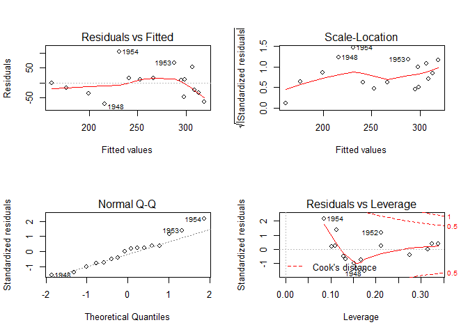
Diagnostic plots
# diagnostic plots
layout ( matrix ( c ( 1 , 2 , 3 , 4 ), 2 , 2 )) # optional 4 graphs/page
plot ( fit )
layout ( matrix ( c ( 1 , 1 , 1 , 1 ), 2 , 2 ))
Comparing two models with ANOVA
# compare models
fit1 <- lm ( y ~ x1 + x2 + x3 + x4 , data = mydata )
fit2 <- lm ( y ~ x1 + x2 )
anova ( fit1 , fit2 )
# compare models
fit1 <- lm ( Armed.Forces ~ GNP + Population , data = longley )
fit2 <- lm ( Armed.Forces ~ GNP , data = longley )
anova ( fit1 , fit2 )
## Analysis of Variance Table
##
## Model 1: Armed.Forces ~ GNP + Population
## Model 2: Armed.Forces ~ GNP
## Res.Df RSS Df Sum of Sq F Pr(>F)
## 1 13 33226
## 2 14 58167 -1 -24941 9.7583 0.008068 **
## ---
## Signif. codes: 0 '***' 0.001 '**' 0.01 '*' 0.05 '.' 0.1 ' ' 1
Cross validation
# dataset
library ( DAAG )
data ( houseprices )
head ( houseprices , 3 )
## area bedrooms sale.price
## 9 694 4 192
## 10 905 4 215
## 11 802 4 215
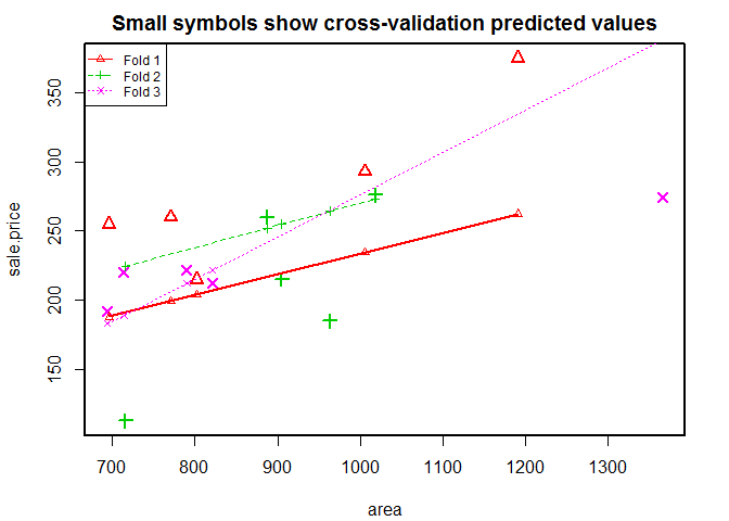
# k-fold cross-validation
library ( DAAG )
# case 1, # 3 fold cross-validation
CVlm ( houseprices , form.lm = formula ( sale.price ~ area ), m = 3 , dots = FALSE , seed = 29 , plotit = c ( "Observed" , "Residual" ), main = "Small symbols show cross-validation predicted values" , legend.pos = "topleft" , printit = TRUE )
## Analysis of Variance Table
##
## Response: sale.price
## Df Sum Sq Mean Sq F value Pr(>F)
## area 1 18566 18566 8 0.014 *
## Residuals 13 30179 2321
## ---
## Signif. codes: 0 '***' 0.001 '**' 0.01 '*' 0.05 '.' 0.1 ' ' 1
1
2
3
4
5
6
7
8
9
10
11
12
13
14
15
16
17
18
19
20
21
22
23
24
25
26
27
28
29
30
31
32
33
34 ##
## fold 1
## Observations in test set: 5
## 11 20 21 22 23
## area 802 696 771.0 1006.0 1191
## cvpred 204 188 199.3 234.7 262
## sale.price 215 255 260.0 293.0 375
## CV residual 11 67 60.7 58.3 113
##
## Sum of squares = 24351 Mean square = 4870 n = 5
##
## fold 2
## Observations in test set: 5
## 10 13 14 17 18
## area 905 716 963.0 1018.00 887.00
## cvpred 255 224 264.4 273.38 252.06
## sale.price 215 113 185.0 276.00 260.00
## CV residual -40 -112 -79.4 2.62 7.94
##
## Sum of squares = 20416 Mean square = 4083 n = 5
##
## fold 3
## Observations in test set: 5
## 9 12 15 16 19
## area 694.0 1366 821.00 714.0 790.00
## cvpred 183.2 388 221.94 189.3 212.49
## sale.price 192.0 274 212.00 220.0 221.50
## CV residual 8.8 -114 -9.94 30.7 9.01
##
## Sum of squares = 14241 Mean square = 2848 n = 5
##
## Overall (Sum over all 5 folds)
## ms
## 3934
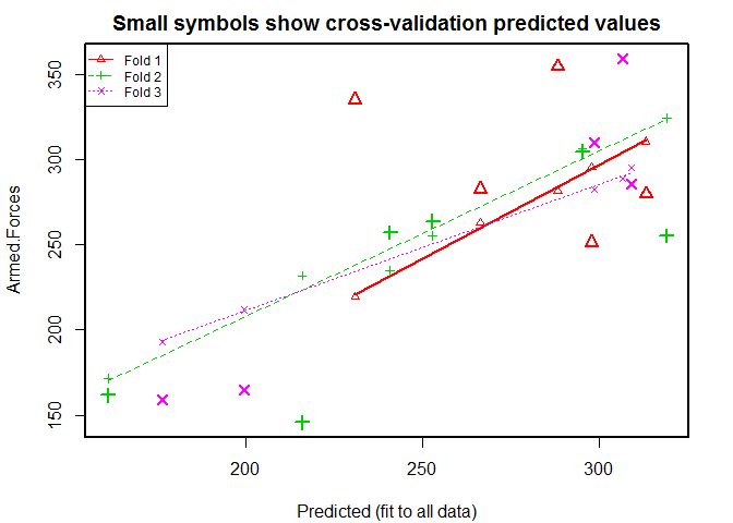
# dataset
head ( longley , 3 )
## GNP.deflator GNP Unemployed Armed.Forces Population Year Employed
## 1947 83.0 234 236 159 108 1947 60.3
## 1948 88.5 259 232 146 109 1948 61.1
## 1949 88.2 258 368 162 110 1949 60.2
# case 2, # 3 fold cross-validation
CVlm ( longley , form.lm = formula ( Armed.Forces ~ GNP + Population ), m = 3 , dots = FALSE , seed = 29 , plotit = c ( "Observed" , "Residual" ), main = "Small symbols show cross-validation predicted values" , legend.pos = "topleft" , printit = TRUE )
## Analysis of Variance Table
##
## Response: Armed.Forces
## Df Sum Sq Mean Sq F value Pr(>F)
## GNP 1 14479 14479 5.66 0.0333 *
## Population 1 24941 24941 9.76 0.0081 **
## Residuals 13 33226 2556
## ---
## Signif. codes: 0 '***' 0.001 '**' 0.01 '*' 0.05 '.' 0.1 ' ' 1
1
2
3
4
5
6
7
8
9
10
11
12
13
14
15
16
17
18
19
20
21
22
23
24
25
26
27
28
29
30
31
32
33
34 ##
## fold 1
## Observations in test set: 5
## 1953 1954 1957 1960 1962
## Predicted 288.1 231 313.0 297.7 266.3
## cvpred 281.4 219 310.6 295.7 263.1
## Armed.Forces 354.7 335 279.8 251.4 282.7
## CV residual 73.3 116 -30.8 -44.3 19.6
##
## Sum of squares = 22004 Mean square = 4401 n = 5
##
## fold 2
## Observations in test set: 6
## 1948 1949 1955 1958 1959 1961
## Predicted 215.9 161.12 295.13 252.78 318.9 240.8
## cvpred 231.9 171.41 306.33 255.07 324.5 234.9
## Armed.Forces 145.6 161.60 304.80 263.70 255.2 257.2
## CV residual -86.3 -9.81 -1.53 8.63 -69.3 22.3
##
## Sum of squares = 12917 Mean square = 2153 n = 6
##
## fold 3
## Observations in test set: 5
## 1947 1950 1951 1952 1956
## Predicted 176.4 199.6 298.5 306.5 308.96
## cvpred 192.8 211.9 282.3 288.9 295.17
## Armed.Forces 159.0 165.0 309.9 359.4 285.70
## CV residual -33.8 -46.9 27.6 70.5 -9.47
##
## Sum of squares = 9161 Mean square = 1832 n = 5
##
## Overall (Sum over all 5 folds)
## ms
## 2755
Variable selection – Heuristic methods
# dataset
head ( longley , 3 )
## GNP.deflator GNP Unemployed Armed.Forces Population Year Employed
## 1947 83.0 234 236 159 108 1947 60.3
## 1948 88.5 259 232 146 109 1948 61.1
## 1949 88.2 258 368 162 110 1949 60.2
# Stepwise Regression
library ( MASS )
fit <- lm ( Armed.Forces ~ GNP + Population + Employed + Unemployed , data = longley )
step <- stepAIC ( fit , direction = "both" )
## Start: AIC=125
## Armed.Forces ~ GNP + Population + Employed + Unemployed
##
## Df Sum of Sq RSS AIC
## <none> 21655 125
## - Unemployed 1 4508 26163 126
## - Population 1 5522 27177 127
## - Employed 1 10208 31863 130
## - GNP 1 15323 36978 132
step $ anova # display results
1
2
3
4
5
6
7
8
9
10
11
12 ## Stepwise Model Path
## Analysis of Deviance Table
##
## Initial Model:
## Armed.Forces ~ GNP + Population + Employed + Unemployed
##
## Final Model:
## Armed.Forces ~ GNP + Population + Employed + Unemployed
##
##
## Step Df Deviance Resid. Df Resid. Dev AIC
## 1 11 21655 125
The goal is to reduce the AIC. Adding variable does not improve the model. Let’s opt for the most valuable variable.
fit <- lm ( Armed.Forces ~ Unemployed , data = longley )
step <- stepAIC ( fit , direction = "both" )
1
2
3
4
5
6
7
8
9
10
11
12
13 ## Start: AIC=138
## Armed.Forces ~ Unemployed
##
## Df Sum of Sq RSS AIC
## - Unemployed 1 2287 72646 137
## <none> 70359 138
##
## Step: AIC=137
## Armed.Forces ~ 1
##
## Df Sum of Sq RSS AIC
## <none> 72646 137
## + Unemployed 1 2287 70359 138
step $ anova # display results
1
2
3
4
5
6
7
8
9
10
11
12
13 ## Stepwise Model Path
## Analysis of Deviance Table
##
## Initial Model:
## Armed.Forces ~ Unemployed
##
## Final Model:
## Armed.Forces ~ 1
##
##
## Step Df Deviance Resid. Df Resid. Dev AIC
## 1 14 70359 138
## 2 - Unemployed 1 2287 15 72646 137
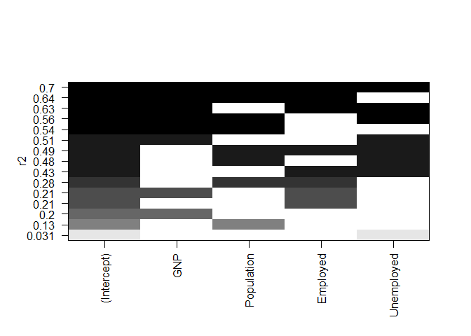
Variable selection – Graphical methods
# model
fit <- lm ( Armed.Forces ~ GNP + Population + Employed + Unemployed , data = longley )
# all Subsets Regression
library ( leaps )
leaps <- regsubsets ( Armed.Forces ~ GNP + Population + Employed + Unemployed , data = longley , nbest = 10 )
# view results
summary ( leaps )
1
2
3
4
5
6
7
8
9
10
11
12
13
14
15
16
17
18
19
20
21
22
23
24
25
26
27 ## Subset selection object
## Call: regsubsets . formula ( Armed . Forces ~ GNP + Population + Employed +
## Unemployed , data = longley , nbest = 10 )
## 4 Variables ( and intercept )
## Forced in Forced out
## GNP FALSE FALSE
## Population FALSE FALSE
## Employed FALSE FALSE
## Unemployed FALSE FALSE
## 10 subsets of each size up to 4
## Selection Algorithm: exhaustive
## GNP Population Employed Unemployed
## 1 ( 1 ) " " " " "*" " "
## 1 ( 2 ) "*" " " " " " "
## 1 ( 3 ) " " "*" " " " "
## 1 ( 4 ) " " " " " " "*"
## 2 ( 1 ) "*" "*" " " " "
## 2 ( 2 ) "*" " " " " "*"
## 2 ( 3 ) " " "*" " " "*"
## 2 ( 4 ) " " " " "*" "*"
## 2 ( 5 ) " " "*" "*" " "
## 2 ( 6 ) "*" " " "*" " "
## 3 ( 1 ) "*" "*" "*" " "
## 3 ( 2 ) "*" " " "*" "*"
## 3 ( 3 ) "*" "*" " " "*"
## 3 ( 4 ) " " "*" "*" "*"
## 4 ( 1 ) "*" "*" "*" "*"
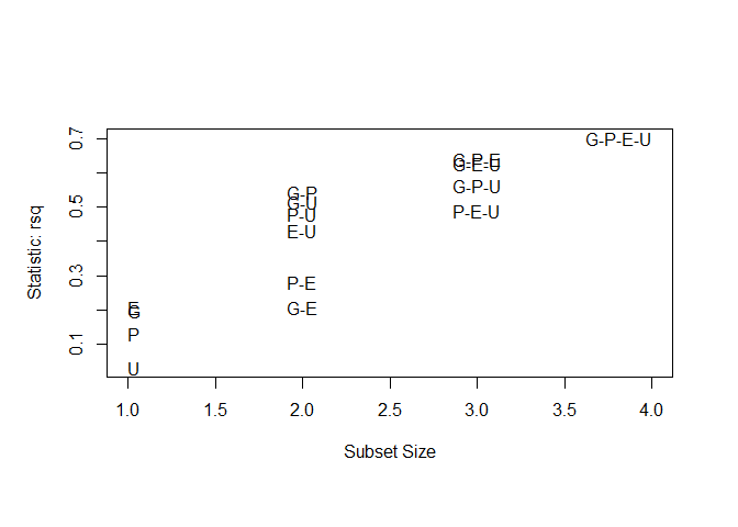
# plot a table of models showing variables in each model
# models are ordered by the selection statistic
plot ( leaps , scale = "r2" )
# plot statistic by subset size
library ( car )
subsets ( leaps , statistic = "rsq" , legend = FALSE ) # available criteria are rsq, rss, adjr2, cp, bic
## Abbreviation
## GNP G
## Population P
## Employed E
## Unemployed U
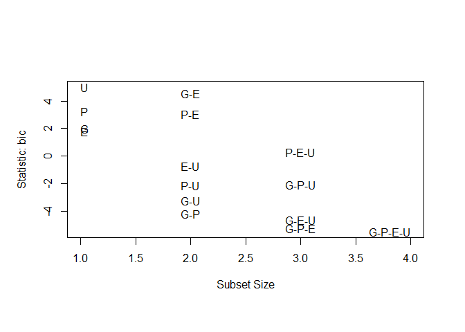
subsets ( leaps , statistic = "bic" , legend = FALSE ) # available criteria are rsq, rss, adjr2, cp, bic
## Abbreviation
## GNP G
## Population P
## Employed E
## Unemployed U
Variable selection – Relative importance
Model: fit <- lm(Armed.Forces ~ GNP + Population + Employed + Unemployed, data = longley).
Warning: eval=FALSE.
# calculate the relative importance of each predictor
library ( relaimpo )
calc.relimp ( fit , type = c ( "lmg" , "last" , "first" , "pratt" ), rela = TRUE )
Results.
1
2
3
4
5
6
7
8
9
10
11
12
13
14
15
16
17
18
19
20
21
22
23
24 Response variable : Armed . Forces
Total response variance : 4843
Analysis based on 16 observations
4 Regressors :
GNP Population Employed Unemployed
Proportion of variance explained by model : 70.2 %
Metrics are normalized to sum to 100 % ( rela = TRUE ) .
Relative importance metrics :
lmg last first pratt
GNP 0.328 0.431 0.348 4.566
Population 0.241 0.155 0.232 - 1.934
Employed 0.217 0.287 0.365 - 1.780
Unemployed 0.215 0.127 0.055 0.148
Average coefficients for different model sizes :
1 X 2 Xs 3 Xs 4 Xs
GNP 0.313 1.301 3.641 5.026
Population 3.646 - 14.815 - 24.637 - 37.260
Employed 9.062 17.646 - 34.249 - 54.144
Unemployed - 0.132 - 0.511 - 0.584 - 0.436
Bootstrapping
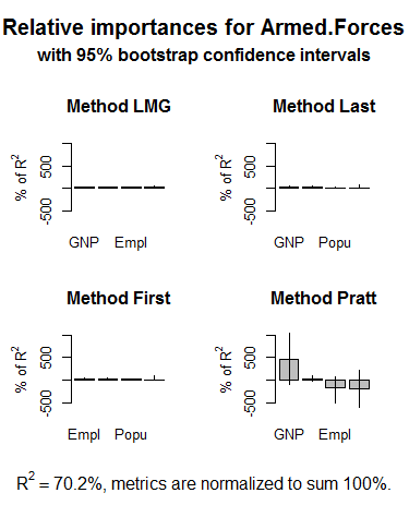
Model: fit <- lm(Armed.Forces ~ GNP + Population + Employed + Unemployed, data = longley).
Warning: eval=FALSE.
# bootstrap measures of relative importance (1000 samples)
boot <- boot.relimp ( fit , b = 1000 , type = c ( "lmg" , "last" , "first" , "pratt" ), rank = TRUE , diff = TRUE , rela = TRUE )
booteval.relimp ( boot ) # print result
Results.
 1
 2
 3
 4
 5
 6
 7
 8
 9
10
11
12
13
14
15
16
17
18
19
20
21
22
23
24
25
26
27
28
29
30
31
32
33
34
35
36
37
38
39
40
41
42
43
44
45
46
47
48
49
50
51
52
53
54
55
56
57
58
59
60
61
62
63
64
65
66
67
68
69
70
71
72
73
74
75
76
77
78
79
80
81
82
83
84
85
86
87
88
89
90 Response variable : Armed . Forces
Total response variance : 4843
Analysis based on 16 observations
4 Regressors :
GNP Population Employed Unemployed
Proportion of variance explained by model : 70.2 %
Metrics are normalized to sum to 100 % ( rela = TRUE ) .
Relative importance metrics :
lmg last first pratt
GNP 0.328 0.431 0.348 4.566
Population 0.241 0.155 0.232 - 1.934
Employed 0.217 0.287 0.365 - 1.780
Unemployed 0.215 0.127 0.055 0.148
Average coefficients for different model sizes :
1 X 2 Xs 3 Xs 4 Xs
GNP 0.313 1.301 3.641 5.026
Population 3.646 - 14.815 - 24.637 - 37.260
Employed 9.062 17.646 - 34.249 - 54.144
Unemployed - 0.132 - 0.511 - 0.584 - 0.436
Confidence interval information ( 1000 bootstrap replicates , bty = perc ):
Relative Contributions with confidence intervals :
Lower Upper
percentage 0.95 0.95 0.95
GNP . lmg 0.3280 ABC_ 0.1488 0.4030
Population . lmg 0.2410 _BCD 0.1572 0.3060
Employed . lmg 0.2170 ABCD 0.1107 0.3240
Unemployed . lmg 0.2150 ABCD 0.0586 0.5550
GNP . last 0.4310 ABCD 0.0101 0.5660
Population . last 0.1550 _BCD 0.0003 0.3850
Employed . last 0.2870 ABCD 0.0476 0.6280
Unemployed . last 0.1270 ABCD 0.0009 0.7810
GNP . first 0.3480 ABCD 0.0151 0.3960
Population . first 0.2320 _BCD 0.0070 0.3060
Employed . first 0.3650 ABCD 0.0159 0.4020
Unemployed . first 0.0550 ABCD 0.0004 0.9280
GNP . pratt 4.5660 ABCD - 1.0160 10.5380
Population . pratt - 1.9340 ABCD - 6.0800 2.2050
Employed . pratt - 1.7800 _BCD - 5.0290 0.8510
Unemployed . pratt 0.1480 ABC_ - 0.3250 1.0910
Letters indicate the ranks covered by bootstrap CIs .
( Rank bootstrap confidence intervals always obtained by percentile method )
CAUTION : Bootstrap confidence intervals can be somewhat liberal .
Differences between Relative Contributions :
Lower Upper
difference 0.95 0.95 0.95
GNP - Population . lmg 0.0871 - 0.0188 0.1521
GNP - Employed . lmg 0.1106 - 0.0479 0.1949
GNP - Unemployed . lmg 0.1130 - 0.4021 0.3281
Population - Employed . lmg 0.0236 - 0.1091 0.1124
Population - Unemployed . lmg 0.0259 - 0.3904 0.2417
Employed - Unemployed . lmg 0.0023 - 0.4315 0.2295
GNP - Population . last 0.2756 - 0.1062 0.4502
GNP - Employed . last 0.1438 - 0.5564 0.4011
GNP - Unemployed . last 0.3041 - 0.7408 0.5502
Population - Employed . last - 0.1318 - 0.6191 0.2653
Population - Unemployed . last 0.0285 - 0.7382 0.3622
Employed - Unemployed . last 0.1603 - 0.6784 0.4852
GNP - Population . first 0.1161 - 0.0590 0.1736
GNP - Employed . first - 0.0172 - 0.0893 0.0934
GNP - Unemployed . first 0.2930 - 0.9047 0.3766
Population - Employed . first - 0.1333 - 0.2134 0.0688
Population - Unemployed . first 0.1769 - 0.8967 0.2969
Employed - Unemployed . first 0.3102 - 0.8937 0.3823
GNP - Population . pratt 6.4995 - 2.2069 15.7978
GNP - Employed . pratt 6.3461 - 1.3879 15.0093
GNP - Unemployed . pratt 4.4180 - 1.9134 10.6456
Population - Employed . pratt - 0.1534 - 4.1860 5.9691
Population - Unemployed . pratt - 2.0815 - 6.1439 2.2348
Employed - Unemployed . pratt - 1.9281 - 5.2057 0.1725
* indicates that CI for difference does not include 0.
CAUTION : Bootstrap confidence intervals can be somewhat liberal .
Warning: eval=FALSE.
plot ( booteval.relimp ( boot , sort = TRUE )) # to plot the results
The .png file.
Going further
The nls package provides functions for nonlinear regression.
Perform robust regression with the rlm function in the MASS package.
The robust package provides a comprehensive library of robust methods, including regression.
The robustbase package also provides basic robust statistics including model selection methods.
Regression diagnostics
# assume that we are fitting a multiple linear regression
fit <- lm ( mpg ~ disp + hp + wt + drat , data = mtcars )
fit
##
## Call:
## lm(formula = mpg ~ disp + hp + wt + drat, data = mtcars)
##
## Coefficients:
## (Intercept) disp hp wt drat
## 29.14874 0.00382 -0.03478 -3.47967 1.76805
Outliers
library ( car )
# assessing outliers
outlierTest ( fit ) # Bonferonni p-value for most extreme obs
##
## No Studentized residuals with Bonferonni p < 0.05
## Largest |rstudent|:
## rstudent unadjusted p-value Bonferonni p
## Toyota Corolla 2.52 0.0184 0.588
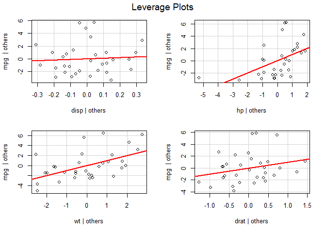
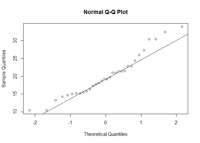
qqPlot ( fit , main = "QQ Plot" ) #qq plot for studentized resid
leveragePlots ( fit ) # leverage plots
Influential observations
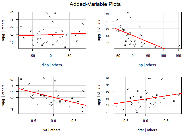
Model: fit <- lm(mpg ~ disp + hp + wt + drat, data = mtcars).
# influential observations
# added variable plots
library ( car )
avPlots ( fit )
par ( mfrow = c ( 1 , 1 ))
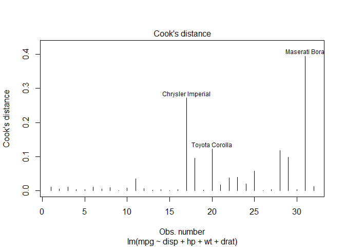
# Cook's D plot
# identify D values > 4/(n-k-1)
cutoff <- 4 / (( nrow ( mtcars ) - length ( fit $ coefficients ) - 2 ))
plot ( fit , which = 4 , cook.levels = cutoff )
Warning: eval=FALSE; interactive function.
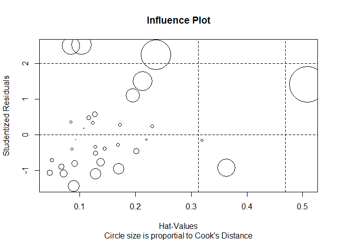
# influence plot
influencePlot ( fit , id.method = "identify" , main = "Influence Plot" , sub = "Circle size is proportial to Cook's Distance" )
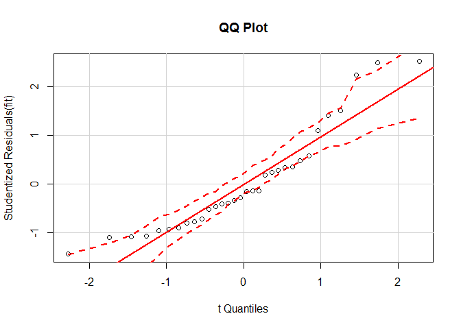
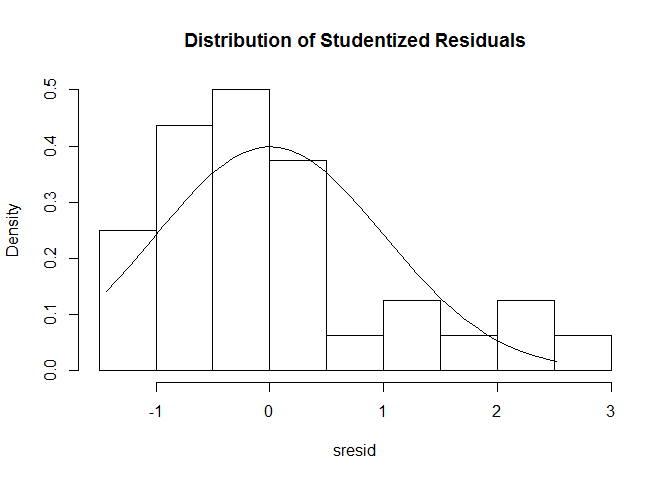
Nonnormality
Model: fit <- lm(mpg ~ disp + hp + wt + drat, data = mtcars).
# normality of residuals
# qq plot for studentized resid
library ( car )
qqPlot ( fit , main = "QQ Plot" )
# distribution of studentized residuals
library ( MASS )
sresid <- studres ( fit )
hist ( sresid , freq = FALSE , main = "Distribution of Studentized Residuals" )
xfit <- seq ( min ( sresid ), max ( sresid ), length = 40 )
yfit <- dnorm ( xfit )
lines ( xfit , yfit )
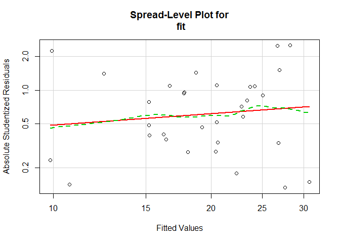
Heteroscedasticity
Nonconstant error variance.
Model: fit <- lm(mpg ~ disp + hp + wt + drat, data = mtcars).
# evaluate homoscedasticity
# non-constant error variance test
ncvTest ( fit )
## Non-constant Variance Score Test
## Variance formula: ~ fitted.values
## Chisquare = 1.43 Df = 1 p = 0.232
# plot studentized residuals vs. fitted values
spreadLevelPlot ( fit )
##
## Suggested power transformation: 0.662
Multicollinearity
Model: fit <- lm(mpg ~ disp + hp + wt + drat, data = mtcars).
# evaluatecCollinearity
vif ( fit )
## disp hp wt drat
## 8.21 2.89 5.10 2.28
sqrt ( vif ( fit )) > 2 # benchmark = 1.96, rounded to 2
## disp hp wt drat
## TRUE FALSE TRUE FALSE
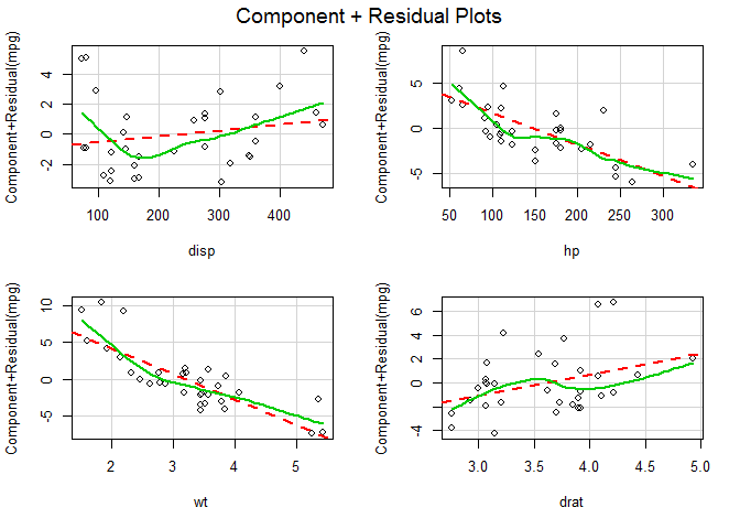
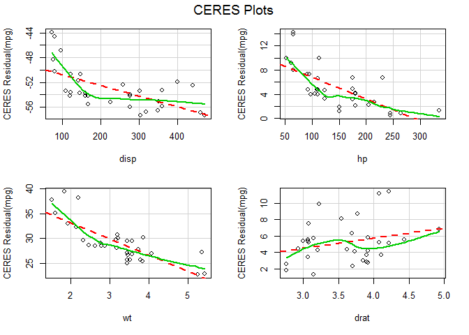
Nonlinearity
Model: fit <- lm(mpg ~ disp + hp + wt + drat, data = mtcars).
# evaluate nonlinearity
# component + residual plot
crPlots ( fit )
# Ceres plots
ceresPlots ( fit )
Autocorrelation
Serial correlation or non-independence of errors.
Model: fit <- lm(mpg ~ disp + hp + wt + drat, data = mtcars).
# test for autocorrelated errors
durbinWatsonTest ( fit )
## lag Autocorrelation D-W Statistic p-value
## 1 0.101 1.74 0.29
## Alternative hypothesis: rho != 0
Global diagnostic
Model: fit <- lm(mpg ~ disp + hp + wt + drat, data = mtcars).
# global test of model assumptions
library ( gvlma )
gvmodel <- gvlma ( fit )
summary ( gvmodel )
1
2
3
4
5
6
7
8
9
10
11
12
13
14
15
16
17
18
19
20
21
22
23
24
25
26
27
28
29
30
31
32
33
34
35
36 ##
## Call:
## lm(formula = mpg ~ disp + hp + wt + drat, data = mtcars)
##
## Residuals:
## Min 1Q Median 3Q Max
## -3.508 -1.905 -0.506 0.982 5.688
##
## Coefficients:
## Estimate Std. Error t value Pr(>|t|)
## (Intercept) 29.14874 6.29359 4.63 8.2e-05 ***
## disp 0.00382 0.01080 0.35 0.7268
## hp -0.03478 0.01160 -3.00 0.0058 **
## wt -3.47967 1.07837 -3.23 0.0033 **
## drat 1.76805 1.31978 1.34 0.1915
## ---
## Signif. codes: 0 '***' 0.001 '**' 0.01 '*' 0.05 '.' 0.1 ' ' 1
##
## Residual standard error: 2.6 on 27 degrees of freedom
## Multiple R-squared: 0.838, Adjusted R-squared: 0.814
## F-statistic: 34.8 on 4 and 27 DF, p-value: 2.7e-10
##
##
## ASSESSMENT OF THE LINEAR MODEL ASSUMPTIONS
## USING THE GLOBAL TEST ON 4 DEGREES-OF-FREEDOM:
## Level of Significance = 0.05
##
## Call:
## gvlma(x = fit)
##
## Value p-value Decision
## Global Stat 13.9382 0.00750 Assumptions NOT satisfied!
## Skewness 4.3131 0.03782 Assumptions NOT satisfied!
## Kurtosis 0.0138 0.90654 Assumptions acceptable.
## Link Function 8.7166 0.00315 Assumptions NOT satisfied!
## Heteroscedasticity 0.8947 0.34421 Assumptions acceptable.
ANOVA
Analysis of variance (ANOVA) is an alternative to regressions among other applications.
# lower case letters are numeric variables
# upper case letters are factors
# one-way ANOVA (completely randomized design)
fit <- aov ( y ~ A , data = mydataframe )
# randomized block design (B is the blocking factor)
fit <- aov ( y ~ A + B , data = mydataframe )
# two-way factorial design
fit <- aov ( y ~ A + B + A : B , data = mydataframe )
fit <- aov ( y ~ A * B , data = mydataframe ) # same thing
# analysis of covariance
fit <- aov ( y ~ A + x , data = mydataframe )
## Grouped Data: uptake ~ conc | Plant
## Plant Type Treatment conc uptake
## 1 Qn1 Quebec nonchilled 95 16.0
## 2 Qn1 Quebec nonchilled 175 30.4
## 3 Qn1 Quebec nonchilled 250 34.8
# one-way ANOVA (completely randomized design)
fit <- aov ( uptake ~ Plant , data = CO2 )
fit
## Call:
## aov(formula = uptake ~ Plant, data = CO2)
##
## Terms:
## Plant Residuals
## Sum of Squares 4862 4845
## Deg. of Freedom 11 72
##
## Residual standard error: 8.2
## Estimated effects are balanced
## Df Sum Sq Mean Sq F value Pr(>F)
## Plant 11 4862 442 6.57 1.8e-07 ***
## Residuals 72 4845 67
## ---
## Signif. codes: 0 '***' 0.001 '**' 0.01 '*' 0.05 '.' 0.1 ' ' 1
# randomized block design (B is the blocking factor)
fit <- aov ( uptake ~ Plant + Type , data = CO2 )
fit
## Call:
## aov(formula = uptake ~ Plant + Type, data = CO2)
##
## Terms:
## Plant Residuals
## Sum of Squares 4862 4845
## Deg. of Freedom 11 72
##
## Residual standard error: 8.2
## 1 out of 13 effects not estimable
## Estimated effects are balanced
## Df Sum Sq Mean Sq F value Pr(>F)
## Plant 11 4862 442 6.57 1.8e-07 ***
## Residuals 72 4845 67
## ---
## Signif. codes: 0 '***' 0.001 '**' 0.01 '*' 0.05 '.' 0.1 ' ' 1
# two-way factorial design
fit <- aov ( uptake ~ Plant + Type + Plant : Type , data = CO2 )
fit
## Call:
## aov(formula = uptake ~ Plant + Type + Plant:Type, data = CO2)
##
## Terms:
## Plant Residuals
## Sum of Squares 4862 4845
## Deg. of Freedom 11 72
##
## Residual standard error: 8.2
## 12 out of 24 effects not estimable
## Estimated effects are balanced
## Df Sum Sq Mean Sq F value Pr(>F)
## Plant 11 4862 442 6.57 1.8e-07 ***
## Residuals 72 4845 67
## ---
## Signif. codes: 0 '***' 0.001 '**' 0.01 '*' 0.05 '.' 0.1 ' ' 1
fit <- aov ( uptake ~ Plant * Type , data = CO2 ) # same thing
fit
## Call:
## aov(formula = uptake ~ Plant * Type, data = CO2)
##
## Terms:
## Plant Residuals
## Sum of Squares 4862 4845
## Deg. of Freedom 11 72
##
## Residual standard error: 8.2
## 12 out of 24 effects not estimable
## Estimated effects are balanced
## Df Sum Sq Mean Sq F value Pr(>F)
## Plant 11 4862 442 6.57 1.8e-07 ***
## Residuals 72 4845 67
## ---
## Signif. codes: 0 '***' 0.001 '**' 0.01 '*' 0.05 '.' 0.1 ' ' 1
# Analysis of Covariance
fit <- aov ( uptake ~ uptake + conc , data = CO2 )
fit
## Call:
## aov(formula = uptake ~ uptake + conc, data = CO2)
##
## Terms:
## conc Residuals
## Sum of Squares 2285 7422
## Deg. of Freedom 1 82
##
## Residual standard error: 9.51
## Estimated effects may be unbalanced
## Df Sum Sq Mean Sq F value Pr(>F)
## conc 1 2285 2285 25.2 2.9e-06 ***
## Residuals 82 7422 91
## ---
## Signif. codes: 0 '***' 0.001 '**' 0.01 '*' 0.05 '.' 0.1 ' ' 1
Evaluate model effects
Type I sequential SS: A+B and B+A will produce different results!
Use the drop1 to produce the familiar Type III results; compare each term with the full model.
# display Type I ANOVA table
fit1 <- aov ( uptake ~ Plant + Type , data = CO2 )
summary ( fit1 )
## Df Sum Sq Mean Sq F value Pr(>F)
## Plant 11 4862 442 6.57 1.8e-07 ***
## Residuals 72 4845 67
## ---
## Signif. codes: 0 '***' 0.001 '**' 0.01 '*' 0.05 '.' 0.1 ' ' 1
# display Type I ANOVA table
fit2 <- aov ( uptake ~ Type + Plant , data = CO2 )
summary ( fit2 )
## Df Sum Sq Mean Sq F value Pr(>F)
## Type 1 3366 3366 50.02 8.1e-10 ***
## Plant 10 1497 150 2.22 0.026 *
## Residuals 72 4845 67
## ---
## Signif. codes: 0 '***' 0.001 '**' 0.01 '*' 0.05 '.' 0.1 ' ' 1
# display type III SS and F tests
drop1 ( fit1 , ~ . , test = "F" )
## Single term deletions
##
## Model:
## uptake ~ Plant + Type
## Df Sum of Sq RSS AIC F value Pr(>F)
## <none> 4845 365
## Plant 10 1497 6341 367 2.22 0.026 *
## Type 0 0 4845 365
## ---
## Signif. codes: 0 '***' 0.001 '**' 0.01 '*' 0.05 '.' 0.1 ' ' 1
drop1 ( fit2 , ~ . , test = "F" )
## Single term deletions
##
## Model:
## uptake ~ Type + Plant
## Df Sum of Sq RSS AIC F value Pr(>F)
## <none> 4845 365
## Type 0 0 4845 365
## Plant 10 1497 6341 367 2.22 0.026 *
## ---
## Signif. codes: 0 '***' 0.001 '**' 0.01 '*' 0.05 '.' 0.1 ' ' 1
Compare nested models directly
fit1 <- aov ( uptake ~ Plant + Type , data = CO2 )
fit2 <- aov ( uptake ~ Plant , data = CO2 )
anova ( fit1 , fit2 )
## Analysis of Variance Table
##
## Model 1: uptake ~ Plant + Type
## Model 2: uptake ~ Plant
## Res.Df RSS Df Sum of Sq F Pr(>F)
## 1 72 4845
## 2 72 4845 0 0
fit2 <- aov ( uptake ~ Plant + Type , data = CO2 )
fit1 <- aov ( uptake ~ Plant , data = CO2 )
anova ( fit1 , fit2 )
## Analysis of Variance Table
##
## Model 1: uptake ~ Plant
## Model 2: uptake ~ Plant + Type
## Res.Df RSS Df Sum of Sq F Pr(>F)
## 1 72 4845
## 2 72 4845 0 0
Multiple comparisons
Tukey HSD tests for post hoc comparisons on each factor in the model.
Factors as an option.
Type I SS.
# model
fit <- aov ( uptake ~ Plant + Type , data = CO2 )
# Tukey honestly significant differences
TukeyHSD ( fit )
1
2
3
4
5
6
7
8
9
10
11
12
13
14
15
16
17
18
19
20
21
22
23
24
25
26
27
28
29
30
31
32
33
34
35
36
37
38
39
40
41
42
43
44
45
46
47
48
49
50
51
52
53
54
55
56
57
58
59
60
61
62
63
64
65
66
67
68
69
70
71
72
73 ## Tukey multiple comparisons of means
## 95% family-wise confidence level
##
## Fit: aov(formula = uptake ~ Plant + Type, data = CO2)
##
## $Plant
## diff lwr upr p adj
## Qn2-Qn1 1.929 -12.88 16.739 1.000
## Qn3-Qn1 4.386 -10.42 19.196 0.997
## Qc1-Qn1 -3.257 -18.07 11.553 1.000
## Qc3-Qn1 -0.643 -15.45 14.168 1.000
## Qc2-Qn1 -0.529 -15.34 14.282 1.000
## Mn3-Qn1 -9.114 -23.92 5.696 0.639
## Mn2-Qn1 -5.886 -20.70 8.925 0.970
## Mn1-Qn1 -6.829 -21.64 7.982 0.918
## Mc2-Qn1 -21.086 -35.90 -6.275 0.000
## Mc3-Qn1 -15.929 -30.74 -1.118 0.024
## Mc1-Qn1 -15.229 -30.04 -0.418 0.038
## Qn3-Qn2 2.457 -12.35 17.268 1.000
## Qc1-Qn2 -5.186 -20.00 9.625 0.989
## Qc3-Qn2 -2.571 -17.38 12.239 1.000
## Qc2-Qn2 -2.457 -17.27 12.353 1.000
## Mn3-Qn2 -11.043 -25.85 3.768 0.346
## Mn2-Qn2 -7.814 -22.62 6.996 0.822
## Mn1-Qn2 -8.757 -23.57 6.053 0.694
## Mc2-Qn2 -23.014 -37.82 -8.204 0.000
## Mc3-Qn2 -17.857 -32.67 -3.047 0.006
## Mc1-Qn2 -17.157 -31.97 -2.347 0.010
## Qc1-Qn3 -7.643 -22.45 7.168 0.842
## Qc3-Qn3 -5.029 -19.84 9.782 0.991
## Qc2-Qn3 -4.914 -19.72 9.896 0.993
## Mn3-Qn3 -13.500 -28.31 1.311 0.108
## Mn2-Qn3 -10.271 -25.08 4.539 0.457
## Mn1-Qn3 -11.214 -26.02 3.596 0.323
## Mc2-Qn3 -25.471 -40.28 -10.661 0.000
## Mc3-Qn3 -20.314 -35.12 -5.504 0.001
## Mc1-Qn3 -19.614 -34.42 -4.804 0.002
## Qc3-Qc1 2.614 -12.20 17.425 1.000
## Qc2-Qc1 2.729 -12.08 17.539 1.000
## Mn3-Qc1 -5.857 -20.67 8.953 0.971
## Mn2-Qc1 -2.629 -17.44 12.182 1.000
## Mn1-Qc1 -3.571 -18.38 11.239 1.000
## Mc2-Qc1 -17.829 -32.64 -3.018 0.006
## Mc3-Qc1 -12.671 -27.48 2.139 0.167
## Mc1-Qc1 -11.971 -26.78 2.839 0.233
## Qc2-Qc3 0.114 -14.70 14.925 1.000
## Mn3-Qc3 -8.471 -23.28 6.339 0.735
## Mn2-Qc3 -5.243 -20.05 9.568 0.988
## Mn1-Qc3 -6.186 -21.00 8.625 0.958
## Mc2-Qc3 -20.443 -35.25 -5.632 0.001
## Mc3-Qc3 -15.286 -30.10 -0.475 0.037
## Mc1-Qc3 -14.586 -29.40 0.225 0.057
## Mn3-Qc2 -8.586 -23.40 6.225 0.719
## Mn2-Qc2 -5.357 -20.17 9.453 0.985
## Mn1-Qc2 -6.300 -21.11 8.511 0.952
## Mc2-Qc2 -20.557 -35.37 -5.747 0.001
## Mc3-Qc2 -15.400 -30.21 -0.589 0.034
## Mc1-Qc2 -14.700 -29.51 0.111 0.054
## Mn2-Mn3 3.229 -11.58 18.039 1.000
## Mn1-Mn3 2.286 -12.52 17.096 1.000
## Mc2-Mn3 -11.971 -26.78 2.839 0.233
## Mc3-Mn3 -6.814 -21.62 7.996 0.919
## Mc1-Mn3 -6.114 -20.92 8.696 0.961
## Mn1-Mn2 -0.943 -15.75 13.868 1.000
## Mc2-Mn2 -15.200 -30.01 -0.389 0.039
## Mc3-Mn2 -10.043 -24.85 4.768 0.493
## Mc1-Mn2 -9.343 -24.15 5.468 0.603
## Mc2-Mn1 -14.257 -29.07 0.553 0.070
## Mc3-Mn1 -9.100 -23.91 5.711 0.641
## Mc1-Mn1 -8.400 -23.21 6.411 0.746
## Mc3-Mc2 5.157 -9.65 19.968 0.989
## Mc1-Mc2 5.857 -8.95 20.668 0.971
## Mc1-Mc3 0.700 -14.11 15.511 1.000
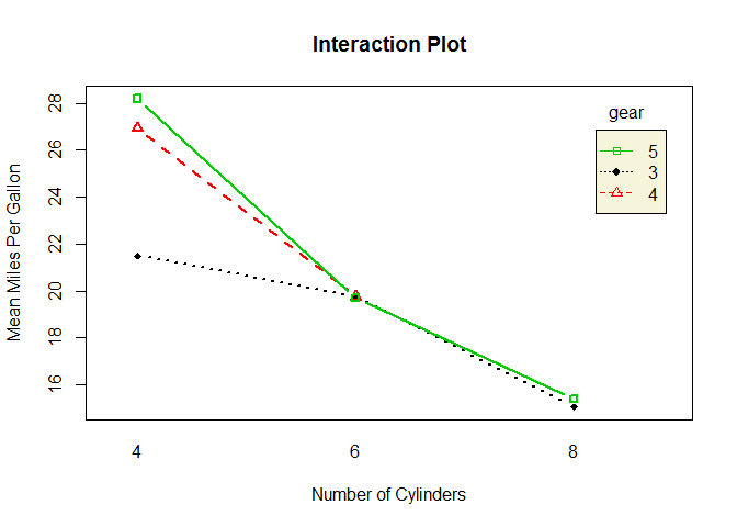
Visualizing results
# two-way interaction plot
attach ( mtcars )
gear <- factor ( gear )
cyl <- factor ( cyl )
# two-way interactions
library ( car )
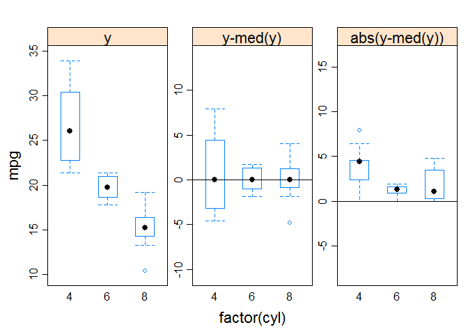
interaction.plot ( cyl , gear , mpg , type = "b" , col = c ( 1 : 3 ), leg.bty = "o" , leg.bg = "beige" , lwd = 2 , pch = c ( 18 , 24 , 22 ), xlab = "Number of Cylinders" , ylab = "Mean Miles Per Gallon" , main = "Interaction Plot" )
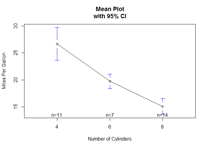
# mean plots for single factors, and includes confidence intervals
library ( gplots )
plotmeans ( mpg ~ cyl , xlab = "Number of Cylinders" , ylab = "Miles Per Gallon" , main = "Mean Plot\nwith 95% CI" )
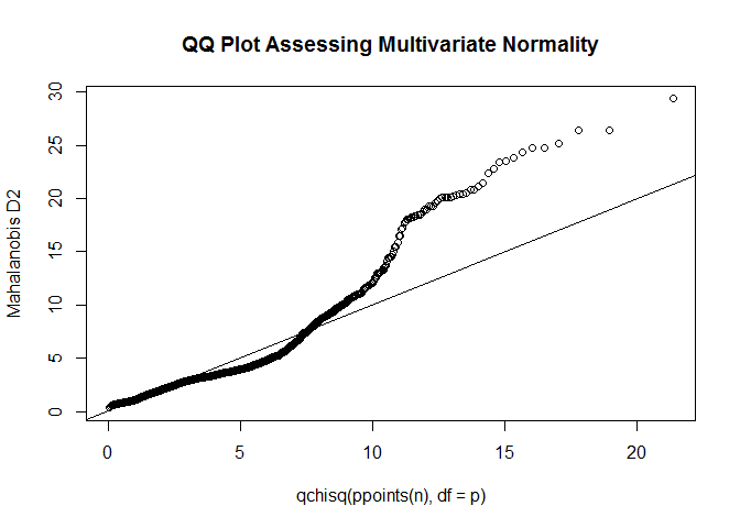
MANOVA
Multivariate analysis of variance (MANOVA) With more than one dependent variable Y. We can run several ANOVA over different Y, or one MANOVA with one Y built with several variables.
## GNP.deflator GNP Unemployed Armed.Forces Population Year Employed
## 1947 83.0 234 236 159 108 1947 60.3
## 1948 88.5 259 232 146 109 1948 61.1
## 1949 88.2 258 368 162 110 1949 60.2
attach ( longley )
# 2x2 factorial MANOVA with 3 dependent variables, Y
Y <- cbind ( Unemployed , Armed.Forces , Employed ) # Y
fit <- manova ( Y ~ Population * GNP ) # Y ~ X
# display type I SS
summary ( fit , test = "Pillai" )
## Df Pillai approx F num Df den Df Pr(>F)
## Population 1 0.997 1074 3 10 7.7e-13 ***
## GNP 1 0.888 26 3 10 4.6e-05 ***
## Population:GNP 1 0.870 22 3 10 9.4e-05 ***
## Residuals 12
## ---
## Signif. codes: 0 '***' 0.001 '**' 0.01 '*' 0.05 '.' 0.1 ' ' 1
# test = "Wilks", "Hotelling-Lawley", and "Roy"
# display univariate statistics
summary.aov ( fit )
1
2
3
4
5
6
7
8
9
10
11
12
13
14
15
16
17
18
19
20
21
22
23
24
25
26 ## Response Unemployed :
## Df Sum Sq Mean Sq F value Pr(>F)
## Population 1 61739 61739 45.92 2e-05 ***
## GNP 1 42841 42841 31.87 0.00011 ***
## Population:GNP 1 10270 10270 7.64 0.01715 *
## Residuals 12 16133 1344
## ---
## Signif. codes: 0 '***' 0.001 '**' 0.01 '*' 0.05 '.' 0.1 ' ' 1
##
## Response Armed.Forces :
## Df Sum Sq Mean Sq F value Pr(>F)
## Population 1 9647 9647 4.25 0.0617 .
## GNP 1 29772 29772 13.10 0.0035 **
## Population:GNP 1 5958 5958 2.62 0.1314
## Residuals 12 27268 2272
## ---
## Signif. codes: 0 '***' 0.001 '**' 0.01 '*' 0.05 '.' 0.1 ' ' 1
##
## Response Employed :
## Df Sum Sq Mean Sq F value Pr(>F)
## Population 1 170.6 170.6 546.45 2.2e-11 ***
## GNP 1 10.5 10.5 33.60 8.5e-05 ***
## Population:GNP 1 0.1 0.1 0.41 0.54
## Residuals 12 3.7 0.3
## ---
## Signif. codes: 0 '***' 0.001 '**' 0.01 '*' 0.05 '.' 0.1 ' ' 1
# display type III SS
fit1 <- manova ( Y ~ Population * GNP )
fit2 <- manova ( Y ~ GNP * Population )
# type III GNP effect
summary ( fit1 )
## Df Pillai approx F num Df den Df Pr(>F)
## Population 1 0.997 1074 3 10 7.7e-13 ***
## GNP 1 0.888 26 3 10 4.6e-05 ***
## Population:GNP 1 0.870 22 3 10 9.4e-05 ***
## Residuals 12
## ---
## Signif. codes: 0 '***' 0.001 '**' 0.01 '*' 0.05 '.' 0.1 ' ' 1
# type III Population effect
summary ( fit2 )
## Df Pillai approx F num Df den Df Pr(>F)
## GNP 1 0.997 1088 3 10 7.2e-13 ***
## Population 1 0.786 12 3 10 0.0011 **
## GNP:Population 1 0.870 22 3 10 9.4e-05 ***
## Residuals 12
## ---
## Signif. codes: 0 '***' 0.001 '**' 0.01 '*' 0.05 '.' 0.1 ' ' 1
Multiple comparisons
TukeyHSD and plot do work with a MANOVA fit. Run each dependent variable separately to obtain them… or proceed with ANOVA on each dependent variable.
Going further
Package lme4 has excellent facilities for fitting linear and generalized linear mixed-effects models.
(M)ANOVA Assumptions
Outliers
Outliers can severely affect normality and homogeneity of variance.
# dataset
head ( mtcars , 3 )
## mpg cyl disp hp drat wt qsec vs am gear carb
## Mazda RX4 21.0 6 160 110 3.90 2.62 16.5 0 1 4 4
## Mazda RX4 Wag 21.0 6 160 110 3.90 2.88 17.0 0 1 4 4
## Datsun 710 22.8 4 108 93 3.85 2.32 18.6 1 1 4 1
# detect outliers
# ordered squared robust Mahalanobis distances of the observations against the empirical distribution function of the MD2i
library ( mvoutlier )
outliers <-
aq.plot ( mtcars [ c ( "mpg" , "disp" , "hp" , "drat" , "wt" , "qsec" )])
## Projection to the first and second robust principal components.
## Proportion of total variation (explained variance): 0.974
outliers # show list of outliers
1
2
3
4
5
6
7
8
9
10
11
12
13
14
15
16
17
18
19
20
21
22
23 ## $outliers
## Mazda RX4 Mazda RX4 Wag Datsun 710
## FALSE FALSE FALSE
## Hornet 4 Drive Hornet Sportabout Valiant
## FALSE FALSE FALSE
## Duster 360 Merc 240D Merc 230
## TRUE TRUE TRUE
## Merc 280 Merc 280C Merc 450SE
## FALSE FALSE FALSE
## Merc 450SL Merc 450SLC Cadillac Fleetwood
## FALSE FALSE FALSE
## Lincoln Continental Chrysler Imperial Fiat 128
## FALSE FALSE TRUE
## Honda Civic Toyota Corolla Toyota Corona
## FALSE FALSE FALSE
## Dodge Challenger AMC Javelin Camaro Z28
## FALSE FALSE TRUE
## Pontiac Firebird Fiat X1-9 Porsche 914-2
## FALSE FALSE FALSE
## Lotus Europa Ford Pantera L Ferrari Dino
## FALSE TRUE FALSE
## Maserati Bora Volvo 142E
## TRUE FALSE
Univariate normality
# Q-Q plot
qqnorm ( mtcars $ mpg )
qqline ( mtcars $ mpg )
# Shapiro-Wilk test of normality
shapiro.test ( mtcars $ mpg )
##
## Shapiro-Wilk normality test
##
## data: mtcars$mpg
## W = 0.9, p-value = 0.1
library ( nortest )
# Anderson-Darling test for normality
ad.test ( mtcars $ mpg )
##
## Anderson-Darling normality test
##
## data: mtcars$mpg
## A = 0.6, p-value = 0.1
# Cramer-von Mises test for normality
cvm.test ( mtcars $ mpg )
##
## Cramer-von Mises normality test
##
## data: mtcars$mpg
## W = 0.09, p-value = 0.2
# Lilliefors (Kolmogorov-Smirnov) test for normality
lillie.test ( mtcars $ mpg )
##
## Lilliefors (Kolmogorov-Smirnov) normality test
##
## data: mtcars$mpg
## D = 0.1, p-value = 0.2
# Pearson chi-square test for normality
pearson.test ( mtcars $ mpg )
##
## Pearson chi-square normality test
##
## data: mtcars$mpg
## P = 8, p-value = 0.2
# Shapiro-Francia test for normality
sf.test ( mtcars $ mpg )
##
## Shapiro-Francia normality test
##
## data: mtcars$mpg
## W = 1, p-value = 0.1
Multivariate normality
## DAX SMI CAC FTSE
## [1,] 1629 1678 1773 2444
## [2,] 1614 1688 1750 2460
## [3,] 1607 1679 1718 2448
library ( mvnormtest )
# Shapiro-Wilk test for multivariate normality of numeric matrix
mshapiro.test ( t ( EuStockMarkets ))
##
## Shapiro-Wilk normality test
##
## data: Z
## W = 0.9, p-value <2e-16
With a p x 1 multivariate normal random vector x vector, the squared Mahalanobis distance between x and ?? is going to be chi-square distributed with p degrees of freedom.
# graphical assessment of multivariate normality
x <- as.matrix ( EuStockMarkets ) # n x p numeric matrix
center <- colMeans ( x ) # centroid
n <- nrow ( x ); p <- ncol ( x )
cov <- cov ( x )
d <- mahalanobis ( x , center , cov ) # distances
qqplot ( qchisq ( ppoints ( n ), df = p ), d , main = "QQ Plot Assessing Multivariate Normality" , ylab = "Mahalanobis D2" )
abline ( a = 0 , b = 1 )
Heteroscedasticity
Nonconstant error variance or non-homogeneity of variances.
# dataset
head ( mtcars , 3 )
## mpg cyl disp hp drat wt qsec vs am gear carb
## Mazda RX4 21.0 6 160 110 3.90 2.62 16.5 0 1 4 4
## Mazda RX4 Wag 21.0 6 160 110 3.90 2.88 17.0 0 1 4 4
## Datsun 710 22.8 4 108 93 3.85 2.32 18.6 1 1 4 1
# y is a numeric variable and G is the grouping variable
# Bartlett parametric test of homogeneity of variances
bartlett.test ( mpg ~ cyl , data = mtcars )
##
## Bartlett test of homogeneity of variances
##
## data: mpg by cyl
## Bartlett's K-squared = 8, df = 2, p-value = 0.02
# Figner-Killeen non-parametric test of homogeneity of variances
fligner.test ( mpg ~ cyl , data = mtcars )
##
## Fligner-Killeen test of homogeneity of variances
##
## data: mpg by cyl
## Fligner-Killeen:med chi-squared = 7, df = 2, p-value = 0.03
library ( HH )
# y is numeric and G is a grouping factor
# G must be of type factor
hov ( mpg ~ factor ( cyl ), data = mtcars )
##
## hov: Brown-Forsyth
##
## data: mpg
## F = 6, df:factor(cyl) = 2, df:Residuals = 30, p-value = 0.009
## alternative hypothesis: variances are not identical
# homogeneity of variance plot
# graphic test of homogeneity of variances based on Brown-Forsyth
hovPlot ( mpg ~ factor ( cyl ), data = mtcars )
Non-homogeneity of covariance matrices
## Sepal.Length Sepal.Width Petal.Length Petal.Width Species
## 1 5.1 3.5 1.4 0.2 setosa
## 2 4.9 3.0 1.4 0.2 setosa
## 3 4.7 3.2 1.3 0.2 setosa
## ---
## biotools version 3.0
# Box's M test
# very sensitive to violations of normality, leading to rejection in most typical cases
boxM ( iris [, -5 ], iris [, 5 ])
##
## Box's M-test for Homogeneity of Covariance Matrices
##
## data: iris[, -5]
## Chi-Sq (approx.) = 100, df = 20, p-value <2e-16
Resampling Statistics
Independent k-sample location tests
# dataset
head ( mtcars , 3 )
## mpg cyl disp hp drat wt qsec vs am gear carb
## Mazda RX4 21.0 6 160 110 3.90 2.62 16.5 0 1 4 4
## Mazda RX4 Wag 21.0 6 160 110 3.90 2.88 17.0 0 1 4 4
## Datsun 710 22.8 4 108 93 3.85 2.32 18.6 1 1 4 1
# exact Wilcoxon Mann Whitney rank sum test
# re-randomization or permutation based statistical tests
# where y is numeric and A is a binary factor
library ( coin )
wilcox_test ( mpg ~ factor ( am ), data = mtcars , distribution = "exact" )
##
## Exact Wilcoxon-Mann-Whitney Test
##
## data: mpg by factor(am) (0, 1)
## Z = -3, p-value = 0.001
## alternative hypothesis: true mu is not equal to 0
# lower case letters represent numerical variables and upper case letters represent categorical factors
Monte-Carlo simulations are available for all tests. Exact tests are available for 2 group procedures.
These tests do not assume random sampling from well-defined populations. They can be a reasonable alternative to classical procedures when test assumptions can not be met.
# one-way permutation test based on 9999 Monte-Carlo
# resamplings
# y is numeric and A is a categorical factor
library ( coin )
oneway_test ( mpg ~ factor ( am ), data = mtcars , distribution = approximate ( B = 9999 ))
##
## Approximative Two-Sample Fisher-Pitman Permutation Test
##
## data: mpg by factor(am) (0, 1)
## Z = -3, p-value = 5e-04
## alternative hypothesis: true mu is not equal to 0
Symmetry of a response for repeated measurements
# exact Wilcoxon signed rank test
# where y1 and y2 are repeated measures
library ( coin )
wilcoxsign_test ( mpg ~ factor ( am ), data = mtcars , distribution = "exact" )
##
## Exact Wilcoxon-Pratt Signed-Rank Test
##
## data: y by x (pos, neg)
## stratified by block
## Z = 5, p-value = 5e-10
## alternative hypothesis: true mu is not equal to 0
# Freidman Test based on 9999 Monte-Carlo resamplings.
# y is numeric, A is a grouping factor, and B is a
# blocking factor
friedman_test ( y ~ A | B , data = mydata , distribution = approximate ( B = 9999 ))
Independence of two numeric variables
# Spearman Test of independence based on 9999 Monte-Carlo
# resamplings. x and y are numeric variables
library ( coin )
spearman_test ( mpg ~ am , data = mtcars , distribution = approximate ( B = 9999 ))
##
## Approximative Spearman Correlation Test
##
## data: mpg by am
## Z = 3, p-value = 0.001
## alternative hypothesis: true rho is not equal to 0
Independence in contingency tables
## Grouped Data: uptake ~ conc | Plant
##   Plant   Type  Treatment conc uptake
## 1   Qn1 Quebec nonchilled   95   16.0
## 2   Qn1 Quebec nonchilled  175   30.4
## 3   Qn1 Quebec nonchilled  250   34.8
## 4 Qn1 Quebec nonchilled 350 37.2
## 5 Qn1 Quebec nonchilled 500 35.3
## 6 Qn1 Quebec nonchilled 675 39.2
cases <- c ( 4 , 2 , 3 , 1 , 59 )
n <- sum ( cases )
cochran <- data.frame (
diphtheria = factor (
unlist ( rep ( list ( c ( 1 , 1 , 1 , 1 ),
c ( 1 , 1 , 0 , 1 ),
c ( 0 , 1 , 1 , 1 ),
c ( 0 , 1 , 0 , 1 ),
c ( 0 , 0 , 0 , 0 )),
cases ))
),
media = factor ( rep ( LETTERS [ 1 : 4 ], n )),
case = factor ( rep ( seq_len ( n ), each = 4 ))
)
head ( cochran )
## diphtheria media case
## 1 1 A 1
## 2 1 B 1
## 3 1 C 1
## 4 1 D 1
## 5 1 A 2
## 6 1 B 2
# independence in 2-way contingency table based on
# 9999 Monte-Carlo resamplings. A and B are factors
library ( coin )
chisq_test ( Plant ~ Type , data = CO2 , distribution = approximate ( B = 9999 ))
##
## Approximative Linear-by-Linear Association Test
##
## data: Plant (ordered) by Type (Quebec, Mississippi)
## Z = -8, p-value <2e-16
## alternative hypothesis: two.sided
# Cochran-Mantel-Haenzsel Test of 3-way Contingency Table
# based on 9999 Monte-Carlo resamplings. A, B, are factors
# and C is a stratefying factor
mh_test ( diphtheria ~ media | case , data = cochran , distribution = approximate ( B = 9999 ))
##
## Approximative Marginal Homogeneity Test
##
## data: diphtheria by
## media (A, B, C, D)
## stratified by case
## chi-squared = 8, p-value = 0.05
# linear by linear association test based on 9999
# Monte-Carlo resamplings
# A and B are ordered factors
library ( coin )
lbl_test ( Plant ~ Type , data = CO2 , distribution = approximate ( B = 9999 ))
##
## Approximative Linear-by-Linear Association Test
##
## data: Plant (ordered) by Type (Quebec, Mississippi)
## Z = -8, p-value <2e-16
## alternative hypothesis: two.sided
Many other univariate and multivariate tests are possible using the functions in the coin package.