Python in RStudio

The knitr package can execute a variety of language chunks:

• Python,
• SQL, and
• Bash, among others.

For Python, instead of {r}, we begin the code chunk with {python}.

x = 'hello, python world!'
print(x.split(' '))

## ['hello,', 'python', 'world!']

Chunk options echo and results are all valid when using Python.

If the Python code generates raw HTML or LaTeX, the results='asis' option ensures that it is passed straight into the document’s output stream.

def aucarre(x):
    print(x ** 2)
    
a = 3
aucarre(a)

9

By default, the interpreter returned by Sys.which("python") is used to execute the code. We can use a different python interpreter with engine.path"/Users/me/anaconda/bin/python" option.

import sys
print(sys.version)

Data exchange

Exchanging data between R chunks and Python chunks (and between Python chunks) is done via the file system.

With data frames, we can use the feather package.

feather¹ transfer a data frame created with Pandas to R for plotting with ggplot2:

Import the data with Python.

import pandas
import feather

cars = pandas.read_csv("img/mtcars.csv")

feather.write_dataframe(cars, "img/cars.feather")

Read the feather file from R and plot the data frame using ggplot2.

library(feather)

mtcars2 <- read_feather("img/cars.feather")

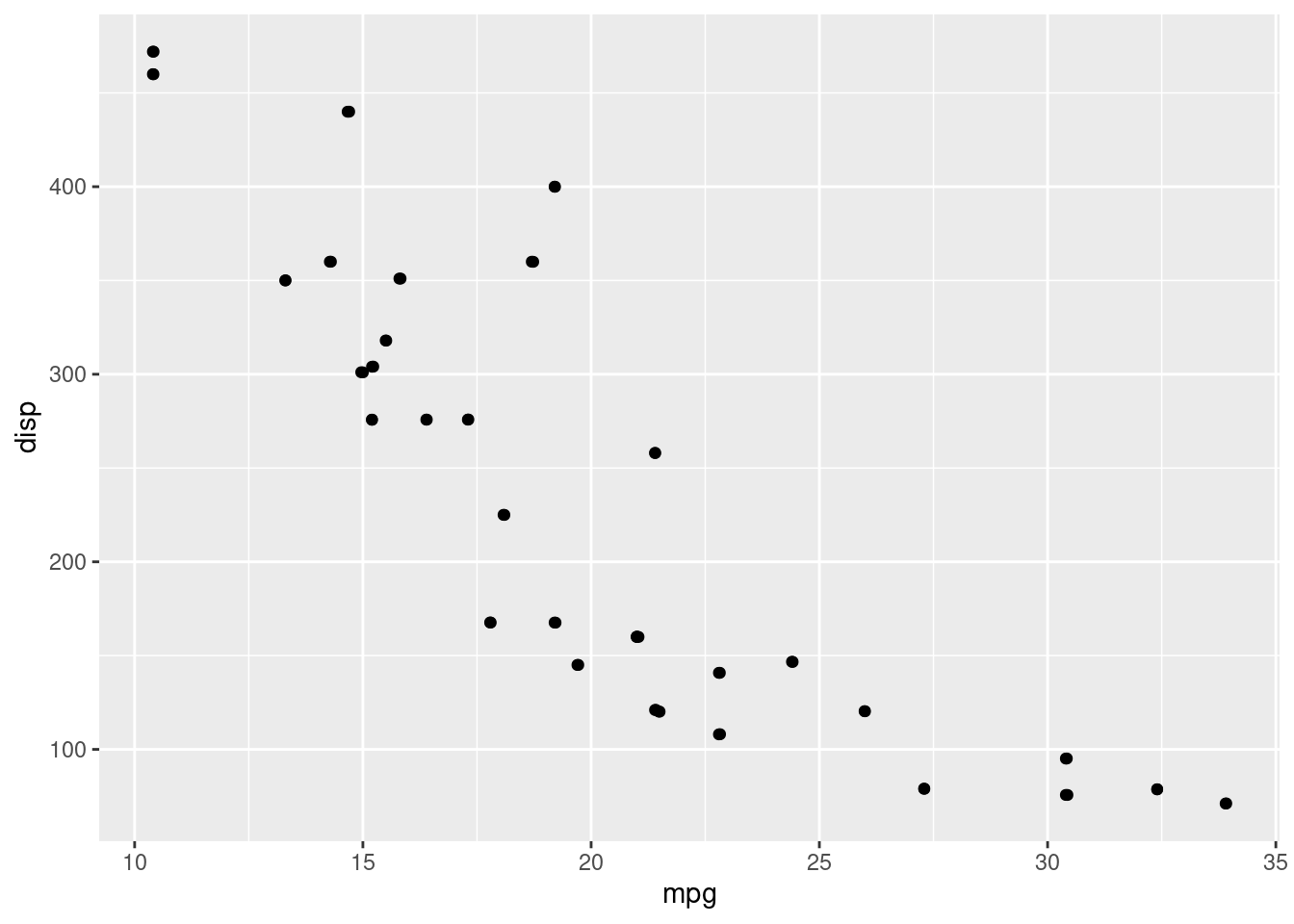
head(mtcars2, 3)

library(ggplot2)

ggplot(mtcars2, aes(mpg, disp)) +
  geom_point() +
  geom_jitter()