EDA, Machine Learning, Feature Engineering, and Kaggle
Foreword
Code snippets and excerpts from the tutorial. Python 3. From DataCamp.
Exploratory Data Analysis (EDA) prior to Machine Learning
Supervised learning models with the help of exploratory data analysis (EDA) on the Titanic data.
How to Start with Supervised Learning (Take 1)
Approach supervised learning is the following:
- Perform an Exploratory Data Analysis (EDA) on a dataset;
- Build a quick and dirty model, or a baseline model, which can serve as a comparison against later models that we will build;
- Iterate this process. We will do more EDA and build another model;
- Engineer features: take the features that we already have and combine them or extract more information from them to eventually come to the last point, which is
- Get a model that performs better.
Import the Data and Explore it
# Import modules
import pandas as pd
import matplotlib.pyplot as plt
import seaborn as sns
from sklearn import tree
from sklearn.metrics import accuracy_score

# Figures inline and set visualization style
%matplotlib inline
sns.set()
# Import test and train datasets
df_train = pd.read_csv('data/train.csv')
df_test = pd.read_csv('data/test.csv')

# View first lines of training data
df_train.head(3)
| PassengerId | Survived | Pclass | Name | Sex | Age | SibSp | Parch | Ticket | Fare | Cabin | Embarked | |
|---|---|---|---|---|---|---|---|---|---|---|---|---|
| 0 | 1 | 0 | 3 | Braund, Mr. Owen Harris | male | 22.0 | 1 | 0 | A/5 21171 | 7.2500 | NaN | S |
| 1 | 2 | 1 | 1 | Cumings, Mrs. John Bradley (Florence Briggs Th... | female | 38.0 | 1 | 0 | PC 17599 | 71.2833 | C85 | C |
| 2 | 3 | 1 | 3 | Heikkinen, Miss. Laina | female | 26.0 | 0 | 0 | STON/O2. 3101282 | 7.9250 | NaN | S |
- The target variable is the variable we are trying to predict;
- Other variables are known as “features” (or “predictor variables”, the features that we are using to predict the target variable).
Note that the df_test DataFrame doesn’t have the Survived column because this is what we will try to predict!
# View first lines of test data
df_test.head(3)
| PassengerId | Pclass | Name | Sex | Age | SibSp | Parch | Ticket | Fare | Cabin | Embarked | |
|---|---|---|---|---|---|---|---|---|---|---|---|
| 0 | 892 | 3 | Kelly, Mr. James | male | 34.5 | 0 | 0 | 330911 | 7.8292 | NaN | Q |
| 1 | 893 | 3 | Wilkes, Mrs. James (Ellen Needs) | female | 47.0 | 1 | 0 | 363272 | 7.0000 | NaN | S |
| 2 | 894 | 2 | Myles, Mr. Thomas Francis | male | 62.0 | 0 | 0 | 240276 | 9.6875 | NaN | Q |
df_train.info()
1 2 3 4 5 6 7 8 9 10 11 12 13 14 15 16 17 | |
df_train.describe()
| PassengerId | Survived | Pclass | Age | SibSp | Parch | Fare | |
|---|---|---|---|---|---|---|---|
| count | 891.000000 | 891.000000 | 891.000000 | 714.000000 | 891.000000 | 891.000000 | 891.000000 |
| mean | 446.000000 | 0.383838 | 2.308642 | 29.699118 | 0.523008 | 0.381594 | 32.204208 |
| std | 257.353842 | 0.486592 | 0.836071 | 14.526497 | 1.102743 | 0.806057 | 49.693429 |
| min | 1.000000 | 0.000000 | 1.000000 | 0.420000 | 0.000000 | 0.000000 | 0.000000 |
| 25% | 223.500000 | 0.000000 | 2.000000 | 20.125000 | 0.000000 | 0.000000 | 7.910400 |
| 50% | 446.000000 | 0.000000 | 3.000000 | 28.000000 | 0.000000 | 0.000000 | 14.454200 |
| 75% | 668.500000 | 1.000000 | 3.000000 | 38.000000 | 1.000000 | 0.000000 | 31.000000 |
| max | 891.000000 | 1.000000 | 3.000000 | 80.000000 | 8.000000 | 6.000000 | 512.329200 |
Visual Exploratory Data Analysis (EDA) and a First Model
With seaborn.
sns.countplot(x='Survived', data=df_train)
1 | |
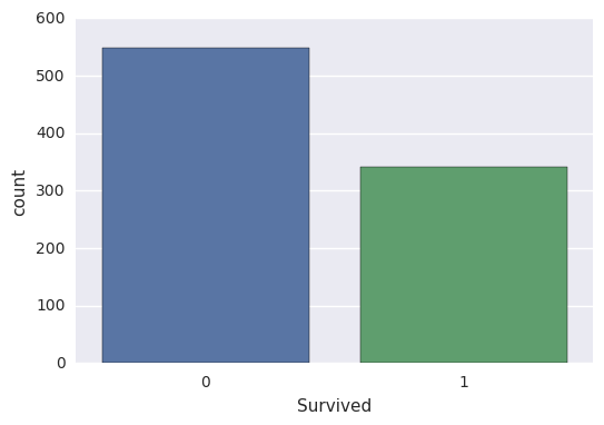
Take-away: in the training set, less people survived than didn’t. Let’s then build a first model that predicts that nobody survived.
This is a bad model as we know that people survived. But it gives us a baseline: any model that we build later needs to do better than this one.
- Create a column
Survivedfordf_testthat encodes ‘did not survive’ for all rows; - Save
PassengerIdandSurvivedcolumns ofdf_testto a .csv and submit to Kaggle.
df_test['Survived'] = 0
df_test[['PassengerId', 'Survived']].to_csv('results/no_survivors.csv', index=False)
Submit to Kaggle (1st)
- Go to Kaggle, log in, and search for Titanic: Machine Learning from Disaster.
- Join the competition and submit the .csv file.
- Add a description and submit.
- Kaggle returns a ranking.
- At the time of the first submission: score 0.63679, rank 9387.

EDA on Feature Variables
Do some more Exploratory Data Analysis and build another model!
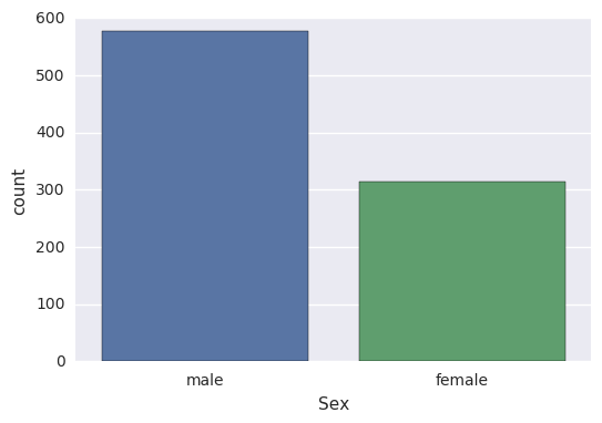
sns.countplot(x='Sex', data=df_train);
# kind is the facets
sns.factorplot(x='Survived', col='Sex', kind='count', data=df_train)
1 | |
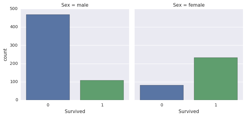
Take-away: Women were more likely to survive than men.
With this take-away, we can use pandas to figure out how many women and how many men survived:
df_train.head(1)
| PassengerId | Survived | Pclass | Name | Sex | Age | SibSp | Parch | Ticket | Fare | Cabin | Embarked | |
|---|---|---|---|---|---|---|---|---|---|---|---|---|
| 0 | 1 | 0 | 3 | Braund, Mr. Owen Harris | male | 22.0 | 1 | 0 | A/5 21171 | 7.25 | NaN | S |
# Chain a group by Sex, sum Survived
df_train.groupby(['Sex']).Survived.sum()
1 2 3 4 | |
# Chain calculations
print(df_train[df_train.Sex == 'female'].Survived.sum() /
      df_train[df_train.Sex == 'female'].Survived.count())

print(df_train[df_train.Sex == 'male'].Survived.sum() /
      df_train[df_train.Sex == 'male'].Survived.count())
1 2 | |
74% of women survived, while 19% of men survived.
Build a second model and predict that all women survived and all men didn’t.
- Create a column
Survivedfordf_testthat encodes the above prediction. - Save
PassengerIdandSurvivedcolumns ofdf_testto a .csv and submit to Kaggle.
df_test['Survived'] = df_test.Sex == 'female'
df_test['Survived'] = df_test.Survived.apply(lambda x: int(x))
df_test.head(3)
| PassengerId | Pclass | Name | Sex | Age | SibSp | Parch | Ticket | Fare | Cabin | Embarked | Survived | |
|---|---|---|---|---|---|---|---|---|---|---|---|---|
| 0 | 892 | 3 | Kelly, Mr. James | male | 34.5 | 0 | 0 | 330911 | 7.8292 | NaN | Q | 0 |
| 1 | 893 | 3 | Wilkes, Mrs. James (Ellen Needs) | female | 47.0 | 1 | 0 | 363272 | 7.0000 | NaN | S | 1 |
| 2 | 894 | 2 | Myles, Mr. Thomas Francis | male | 62.0 | 0 | 0 | 240276 | 9.6875 | NaN | Q | 0 |
df_test[['PassengerId', 'Survived']].to_csv('results/women_survived.csv', index=False)
Submit to Kaggle (2nd)
- Go to Kaggle, log in, and search for Titanic: Machine Learning from Disaster.
- Join the competition and submit the .csv file.
- Add a description and submit.
- Kaggle returns a ranking.
- At the time of the first submission: score 0.76555 (from 0.62679), rank 7274 (a jump of 2122 places).

Explore the Data More!
# kind is the facets
sns.factorplot(x='Survived', col='Pclass', kind='count', data=df_train)
1 | |

Take-away: Passengers that travelled in first class were more likely to survive. On the other hand, passengers travelling in third class were more unlikely to survive.
# kind is the facets
sns.factorplot(x='Survived', col='Embarked', kind='count', data=df_train)
1 | |
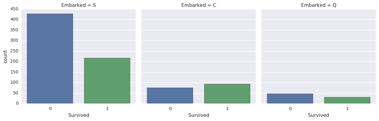
Take-away: Passengers that embarked in Southampton were less likely to survive.
EDA with Numeric Variables
sns.distplot(df_train.Fare, kde=False)
1 | |
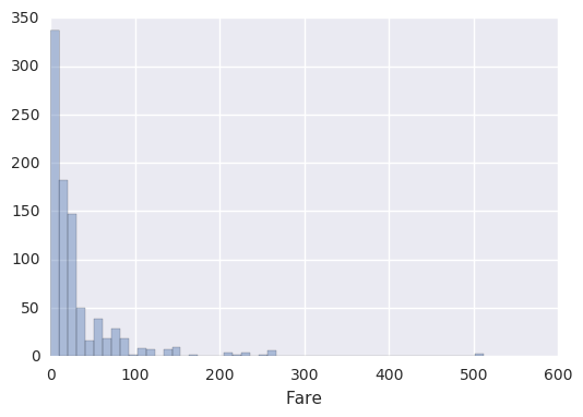
Take-away: Most passengers paid less than 100 for travelling with the Titanic.
# Group by Survived, trace histograms of Fare with alpha color 0.6
df_train.groupby('Survived').Fare.hist(alpha=0.6)
1 2 3 4 | |

Take-away: It looks as though those that paid more had a higher chance of surviving.
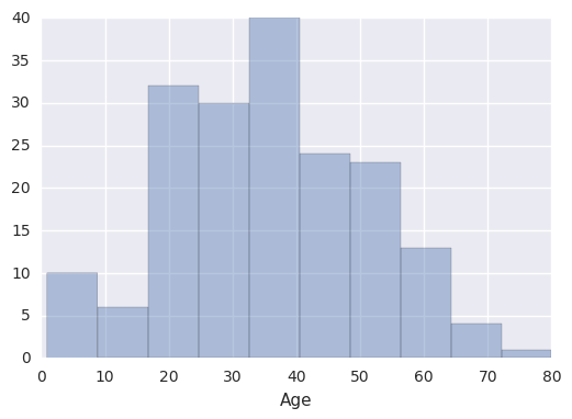
# Remove NaN
df_train_drop = df_train.dropna()

sns.distplot(df_train_drop.Age, kde=False)
1 | |
# Alternative to bars or scatter
sns.stripplot(x='Survived',
              y='Fare',
              data=df_train,
              alpha=0.3, jitter=True)
1 | |

# Alternative to bars or scatter
sns.swarmplot(x='Survived',
              y='Fare',
              data=df_train)
1 | |

Take-away: Fare definitely seems to be correlated with survival aboard the Titanic.
# Group by Survived, describe Fare (descriptive statistics)
df_train.groupby('Survived').Fare.describe()
| count | mean | std | min | 25% | 50% | 75% | max | |
|---|---|---|---|---|---|---|---|---|
| Survived | ||||||||
| 0 | 549.0 | 22.117887 | 31.388207 | 0.0 | 7.8542 | 10.5 | 26.0 | 263.0000 |
| 1 | 342.0 | 48.395408 | 66.596998 | 0.0 | 12.4750 | 26.0 | 57.0 | 512.3292 |
sns.lmplot(x='Age',
           y='Fare',
           hue='Survived',
           data=df_train,
           fit_reg=False, scatter_kws={'alpha':0.5})
1 | |

sns.lmplot(x='Age',
           y='Fare',
           hue='Survived',
           data=df_train,
           fit_reg=True, scatter_kws={'alpha':0.5})
1 | |
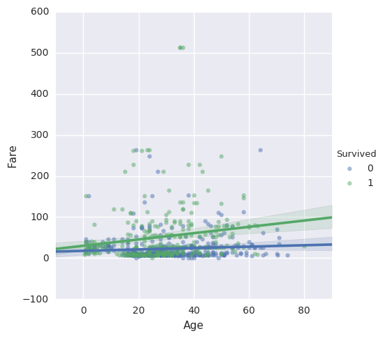
Take-away: It looks like those who survived either paid quite a bit for their ticket or they were young.
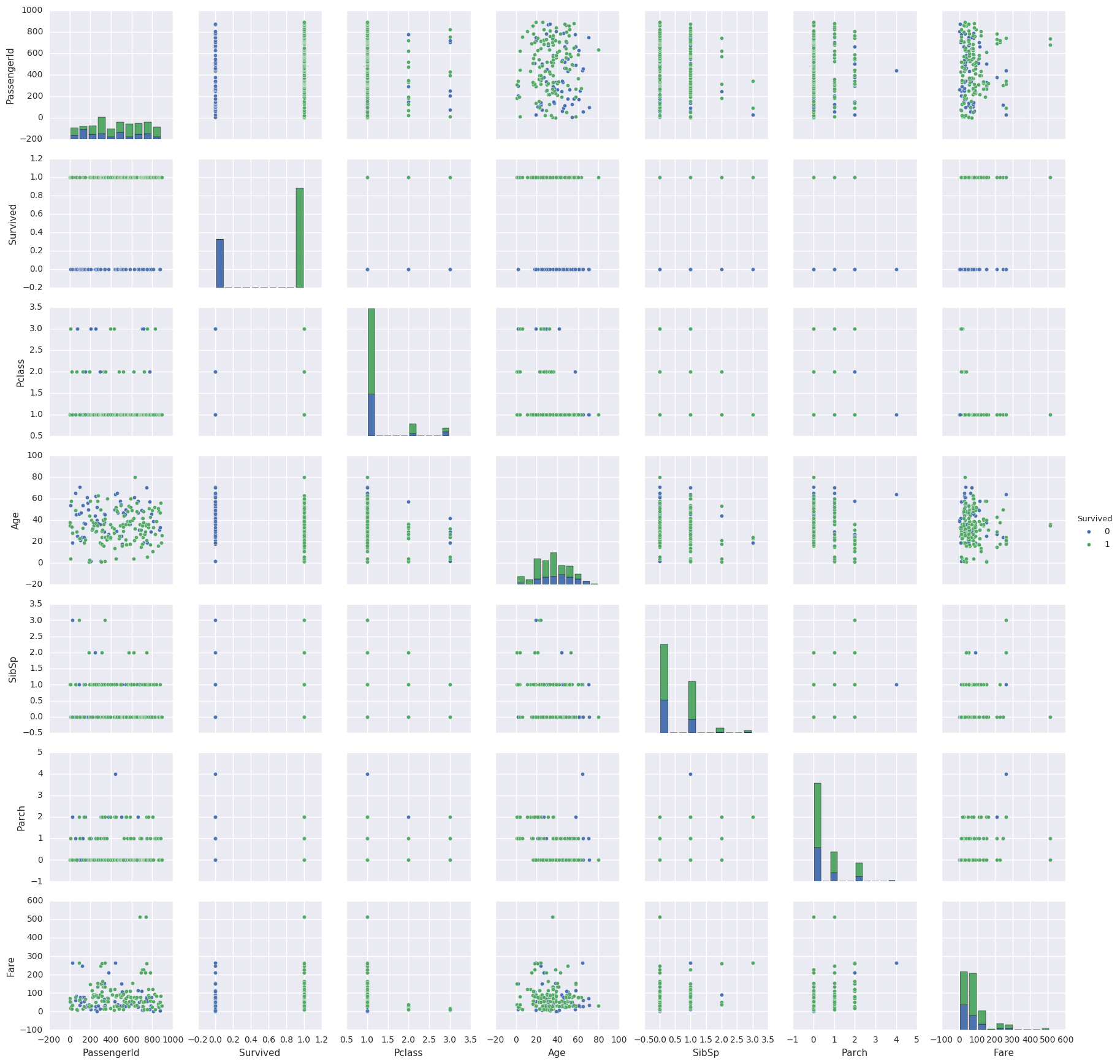
sns.pairplot(df_train_drop, hue='Survived')
1 | |
A First Machine Learning Model
A decision tree classifier, with the Python scikit-learn.
How to Start with Supervised Learning (Take 2)
Now that we have done our homeworks with EDA…
# Import modules
import pandas as pd
import matplotlib.pyplot as plt
import seaborn as sns
import re
import numpy as np
from sklearn import tree
from sklearn.model_selection import train_test_split
from sklearn.linear_model import LogisticRegression
from sklearn.model_selection import GridSearchCV

# Figures inline and set visualization style
%matplotlib inline
sns.set()
# Import data
df_train = pd.read_csv('data/train.csv')
df_test = pd.read_csv('data/test.csv')
df_train.info()
1 2 3 4 5 6 7 8 9 10 11 12 13 14 15 16 17 | |
df_test.info()
1 2 3 4 5 6 7 8 9 10 11 12 13 14 15 16 | |
# Store target variable of training data in a safe place
survived_train = df_train.Survived

# Concatenate (along the index or axis=1) training and test sets
# to preprocess the data a little bit
# and make sure that any operations that
# we perform on the training set are also
# being done on the test data set
data = pd.concat([df_train.drop(['Survived'], axis=1), df_test])
# The combined datasets (891+418 entries)
data.info()
1 2 3 4 5 6 7 8 9 10 11 12 13 14 15 16 | |
Missing values for the Age and Fare columns! Also notice that Cabin and Embarked are also missing values and we will need to deal with that also at some point. However, now we will focus on fixing the numerical variables Age and Fare, using the median of the of these variables where we know them. It’s perfect for dealing with outliers. In other words, the median is useful to use when the distribution of data is skewed. Other ways to impute the missing values would be to use the mean or the mode.
# Impute missing numerical variables where NaN
data['Age'] = data.Age.fillna(data.Age.median())
data['Fare'] = data.Fare.fillna(data.Fare.median())

# Check out info of data
data.info()
1 2 3 4 5 6 7 8 9 10 11 12 13 14 15 16 | |
Encode the data with numbers with .get_dummies().
It creates a new column for female, called Sex_female, and then a new column for Sex_male, which encodes whether that row was male or female (1 if that row is a male - and a 0 if that row is female). Because of drop_first argument, we dropped Sex_female because, essentially, these new columns, Sex_female and Sex_male, encode the same information.
data = pd.get_dummies(data, columns=['Sex'], drop_first=True)
data.head(3)
| PassengerId | Pclass | Name | Age | SibSp | Parch | Ticket | Fare | Cabin | Embarked | Sex_male | |
|---|---|---|---|---|---|---|---|---|---|---|---|
| 0 | 1 | 3 | Braund, Mr. Owen Harris | 22.0 | 1 | 0 | A/5 21171 | 7.2500 | NaN | S | 1 |
| 1 | 2 | 1 | Cumings, Mrs. John Bradley (Florence Briggs Th... | 38.0 | 1 | 0 | PC 17599 | 71.2833 | C85 | C | 0 |
| 2 | 3 | 3 | Heikkinen, Miss. Laina | 26.0 | 0 | 0 | STON/O2. 3101282 | 7.9250 | NaN | S | 0 |
# Select columns and view head
data = data[['Sex_male', 'Fare', 'Age','Pclass', 'SibSp']]
data.head(3)
| Sex_male | Fare | Age | Pclass | SibSp | |
|---|---|---|---|---|---|
| 0 | 1 | 7.2500 | 22.0 | 3 | 1 |
| 1 | 0 | 71.2833 | 38.0 | 1 | 1 |
| 2 | 0 | 7.9250 | 26.0 | 3 | 0 |
data.info()
1 2 3 4 5 6 7 8 9 10 | |
All the entries are non-null now.
Build a Decision Tree Classifier
“Was Sex_male” less than 0.5? In other words, was the data point a female. If the answer to this question is True, we can go down to the left and we get Survived. If False, we go down the right and we get Dead.

That the first branch is on Male or not and that Male results in a prediction of Dead. The gini coefficient is used to make these decisions.
Before fitting a model to the data, split it back into training and test sets:
data_train = data.iloc[:891]
data_test = data.iloc[891:]
scikit-learn requires the data as arrays, not DataFrames. Transform them.
X = data_train.values
test = data_test.values

# and from above: survived_train = df_train.Survived
y = survived_train.values
X
1 2 3 4 5 6 7 | |
Build a decision tree classifier! First create such a model with max_depth=3 and then fit it the data. Name the model clf, which is short for “Classifier”.
# Instantiate model and fit to data
# The max depth is set at 3
clf = tree.DecisionTreeClassifier(max_depth=3)

# X is the indenpendent variables, y is the dependent variable
clf.fit(X, y)
1 2 3 4 5 6 | |
Make predictions on the test set.
# Make predictions and store in 'Survived' column of df_test
Y_pred = clf.predict(test)
df_test['Survived'] = Y_pred

# Save it
df_test[['PassengerId', 'Survived']].to_csv('results/1st_dec_tree.csv',
                                            index=False)
Submit to Kaggle (3rd)
- Go to Kaggle, log in, and search for Titanic: Machine Learning from Disaster.
- Join the competition and submit the .csv file.
- Add a description and submit.
- Kaggle returns a ranking.
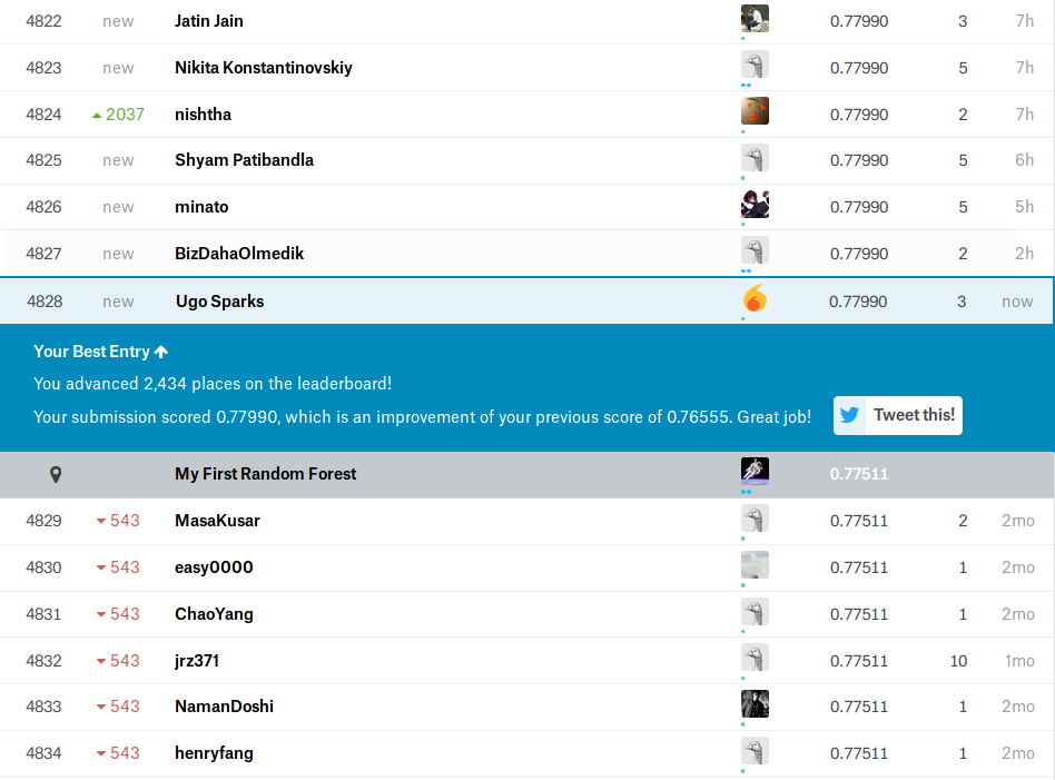
- At the time of the first submission: score 0.77990 (from 0.76555), rank 4828 (a jump of 2434 places).
# Compute accuracy on the training set
train_accuracy = clf.score(X, y)
train_accuracy
1 | |
A Decision Tree Classifier in More Details
The Decision Tree Classifier we just built had a max_depth=3 and it looks like this:
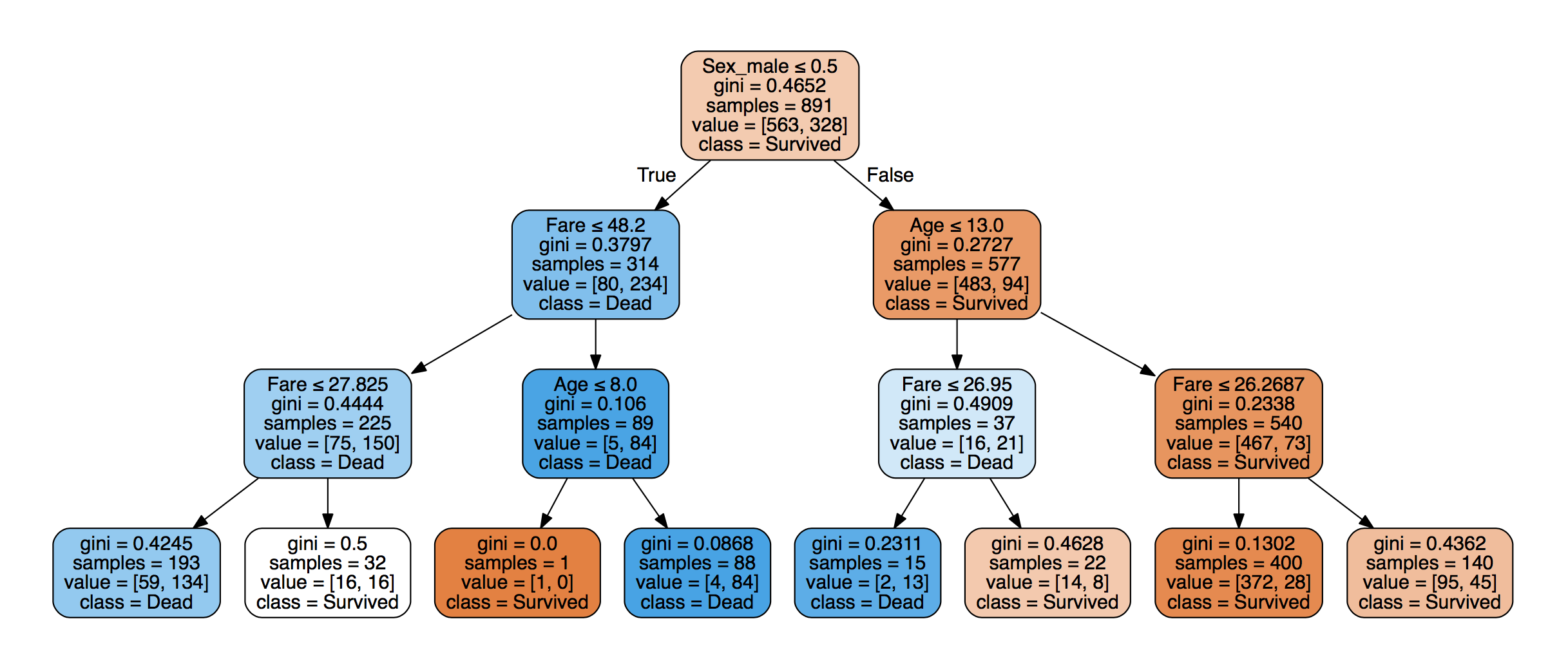
The maximal distance between the first decision and the last is 3, so that’s max_depth=3.
Generate images with graphviz.
import graphviz

tree_data = tree.export_graphviz(clf, out_file=None)
graph = graphviz.Source(tree_data)
# Save the pdf
graph.render("img/tree_data")
1 | |
We get a tree_data test file (the code for generating the image) and a pdf file. We can generate an image.
feature_names = list(data_train)
feature_names
1 | |
#data_train
#data_test
tree_data = tree.export_graphviz(clf, out_file=None,
                                feature_names=feature_names,
                                class_names=None,
                                filled=True, rounded=True,
                                special_characters=True)
graph = graphviz.Source(tree_data)
graph
IN THE NOTEBOOK ONLY!
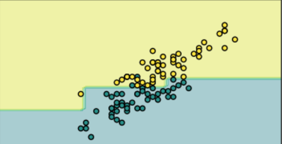
In building this model, what we are essentially doing is creating a decision boundary in the space of feature variables.
Why Choose max_depth=3?
The depth of the tree is known as a hyperparameter, which means a parameter we need to decide before we fit the model to the data. If we choose a larger max_depth, we will get a more complex decision boundary; the bias-variance trade-off.
- If the decision boundary is too complex, we can overfit to the data, which means that the model will be describing noise as well as signal.
- If the
max_depthis too small, we might be underfitting the data, meaning that the model doesn’t contain enough of the signal.
One way is to hold out a test set from the training data. We can then fit the model to the training data, make predictions on the test set and see how well the prediction does on the test set.
Split the original training data into training and test sets:
X_train, X_test, y_train, y_test = train_test_split(X, y, test_size=0.33, random_state=42, stratify=y)
Iterate over values of max_depth ranging from 1 to 9 and plot the accuracy of the models on training and test sets:
# Setup arrays to store train and test accuracies
dep = np.arange(1, 9)
train_accuracy = np.empty(len(dep))
test_accuracy = np.empty(len(dep))

# Loop over different values of k
for i, k in enumerate(dep):
    # Setup a k-NN Classifier with k neighbors: knn
    clf = tree.DecisionTreeClassifier(max_depth=k)

    # Fit the classifier to the training data
    clf.fit(X_train, y_train)

    # Compute accuracy on the training set
    train_accuracy[i] = clf.score(X_train, y_train)

    # Compute accuracy on the testing set
    test_accuracy[i] = clf.score(X_test, y_test)

# Generate plot
plt.title('clf: Varying depth of tree')
plt.plot(dep, test_accuracy, label = 'Testing Accuracy')
plt.plot(dep, train_accuracy, label = 'Training Accuracy')
plt.legend()
plt.xlabel('Depth of tree')
plt.ylabel('Accuracy')
plt.show()

At max_depth-3, we get the same results as with the model before (around 82%).
As we increase the max_depth, we are going to fit better and better to the training data because we will make decisions that describe the training data. The accuracy for the training data will go up and up, but we see that this doesn’t happen for the test data: we are overfitting.
So that’s why we chose max_depth=3.
Feature Engineering
https://www.datacamp.com/community/tutorials/feature-engineering-kaggle
A process where we use domain knowledge of the data to create additional relevant features (create new columns, transform variables and more) that increase the predictive power of the learning algorithm and make the machine learning models perform even better.
How to Start with Feature Engineering
# Imports
import pandas as pd
import matplotlib.pyplot as plt
import seaborn as sns
import re
import numpy as np
from sklearn import tree
from sklearn.model_selection import GridSearchCV

# Figures inline and set visualization style
%matplotlib inline
sns.set()
# Import data
df_train = pd.read_csv('data/train.csv')
df_test = pd.read_csv('data/test.csv')

# Store target variable of training data in a safe place
survived_train = df_train.Survived

# Concatenate training and test sets
data = pd.concat([df_train.drop(['Survived'], axis=1), df_test])

# View head
data.info()
1 2 3 4 5 6 7 8 9 10 11 12 13 14 15 16 | |
Why Feature Engineer At All?
Titanic’s Passenger Titles
# View head of 'Name' column
data.Name.tail()
1 2 3 4 5 6 | |
These titles of course give us information on social status, profession, etc., which in the end could tell us something more about survival. use regular expressions to extract the title and store it in a new column ‘Title’:
# Extract Title from Name, store in column and plot barplot
# One upper character, one lower character, one dot
data['Title'] = data.Name.apply(lambda x: re.search(' ([A-Z][a-z]+)\.', x).group(1))
# New column Title is a new feature of the dataset
data.Title.head(3)
1 2 3 4 | |
sns.countplot(x='Title', data=data);
plt.xticks(rotation=45);

# Substitute some title with their English form
data['Title'] = data['Title'].replace({'Mlle':'Miss', 'Mme':'Mrs', 'Ms':'Miss'})
# Gather exceptions
data['Title'] = data['Title'].replace(['Don', 'Dona', 'Rev', 'Dr', 'Major', 'Lady', 'Sir', 'Col', 'Capt', 'Countess', 'Jonkheer'],'Special')
data.Title.head(3)
1 2 3 4 | |
sns.countplot(x='Title', data=data);
plt.xticks(rotation=45);

# View tail of data (for change)
data.tail(3)
| PassengerId | Pclass | Name | Sex | Age | SibSp | Parch | Ticket | Fare | Cabin | Embarked | Title | |
|---|---|---|---|---|---|---|---|---|---|---|---|---|
| 415 | 1307 | 3 | Saether, Mr. Simon Sivertsen | male | 38.5 | 0 | 0 | SOTON/O.Q. 3101262 | 7.2500 | NaN | S | Mr |
| 416 | 1308 | 3 | Ware, Mr. Frederick | male | NaN | 0 | 0 | 359309 | 8.0500 | NaN | S | Mr |
| 417 | 1309 | 3 | Peter, Master. Michael J | male | NaN | 1 | 1 | 2668 | 22.3583 | NaN | C | Master |
Passenger’s Cabins
There are several NaNs or missing values in the Cabin column. Those NaNs didn’t have a cabin, which could tell us something about survival.
# View head of data
data[['Name', 'PassengerId', 'Ticket', 'Cabin']].head()
| Name | PassengerId | Ticket | Cabin | |
|---|---|---|---|---|
| 0 | Braund, Mr. Owen Harris | 1 | A/5 21171 | NaN |
| 1 | Cumings, Mrs. John Bradley (Florence Briggs Th... | 2 | PC 17599 | C85 |
| 2 | Heikkinen, Miss. Laina | 3 | STON/O2. 3101282 | NaN |
| 3 | Futrelle, Mrs. Jacques Heath (Lily May Peel) | 4 | 113803 | C123 |
| 4 | Allen, Mr. William Henry | 5 | 373450 | NaN |
# Did they have a Cabin?
# Return True is the passenger has a cabin
data['Has_Cabin'] = ~data.Cabin.isnull()

# # View head of data
data[['Name', 'PassengerId', 'Ticket', 'Cabin', 'Has_Cabin']].head()
| Name | PassengerId | Ticket | Cabin | Has_Cabin | |
|---|---|---|---|---|---|
| 0 | Braund, Mr. Owen Harris | 1 | A/5 21171 | NaN | False |
| 1 | Cumings, Mrs. John Bradley (Florence Briggs Th... | 2 | PC 17599 | C85 | True |
| 2 | Heikkinen, Miss. Laina | 3 | STON/O2. 3101282 | NaN | False |
| 3 | Futrelle, Mrs. Jacques Heath (Lily May Peel) | 4 | 113803 | C123 | True |
| 4 | Allen, Mr. William Henry | 5 | 373450 | NaN | False |
Drop these columns, except Has_Cabin, in the actual data DataFrame; make sure to use the inplace argument in the .drop() method and set it to True:
# Drop columns and view head
data.drop(['Cabin', 'Name', 'PassengerId', 'Ticket'], axis=1, inplace=True)
data.head()
| Pclass | Sex | Age | SibSp | Parch | Fare | Embarked | Title | Has_Cabin | |
|---|---|---|---|---|---|---|---|---|---|
| 0 | 3 | male | 22.0 | 1 | 0 | 7.2500 | S | Mr | False |
| 1 | 1 | female | 38.0 | 1 | 0 | 71.2833 | C | Mrs | True |
| 2 | 3 | female | 26.0 | 0 | 0 | 7.9250 | S | Miss | False |
| 3 | 1 | female | 35.0 | 1 | 0 | 53.1000 | S | Mrs | True |
| 4 | 3 | male | 35.0 | 0 | 0 | 8.0500 | S | Mr | False |
New features such as Title and Has_Cabin.
Features that don’t add any more useful information for the machine learning model are now dropped from the DataFrame.
Handling Missing Values
data.info()
1 2 3 4 5 6 7 8 9 10 11 12 13 14 | |
Missing values in Age, Fare, and Embarked. Impute these missing values with the help of .fillna() and use the median to fill in the columns (or the mean, the mode, etc.).
# Impute missing values for Age, Fare, Embarked
data['Age'] = data.Age.fillna(data.Age.median())
data['Fare'] = data.Fare.fillna(data.Fare.median())
data['Embarked'] = data['Embarked'].fillna('S')
data.info()
1 2 3 4 5 6 7 8 9 10 11 12 13 14 | |
data.head(3)
| Pclass | Sex | Age | SibSp | Parch | Fare | Embarked | Title | Has_Cabin | |
|---|---|---|---|---|---|---|---|---|---|
| 0 | 3 | male | 22.0 | 1 | 0 | 7.2500 | S | Mr | False |
| 1 | 1 | female | 38.0 | 1 | 0 | 71.2833 | C | Mrs | True |
| 2 | 3 | female | 26.0 | 0 | 0 | 7.9250 | S | Miss | False |
Binning Numerical Data
# Binning numerical columns
# q=4 means 4 quantiles 0, 1, 2, 3
# labels=False are numbers, not characters
data['CatAge'] = pd.qcut(data.Age, q=4, labels=False )
data['CatFare']= pd.qcut(data.Fare, q=4, labels=False)
data.head(3)
| Pclass | Sex | Age | SibSp | Parch | Fare | Embarked | Title | Has_Cabin | CatAge | CatFare | |
|---|---|---|---|---|---|---|---|---|---|---|---|
| 0 | 3 | male | 22.0 | 1 | 0 | 7.2500 | S | Mr | False | 0 | 0 |
| 1 | 1 | female | 38.0 | 1 | 0 | 71.2833 | C | Mrs | True | 3 | 3 |
| 2 | 3 | female | 26.0 | 0 | 0 | 7.9250 | S | Miss | False | 1 | 1 |
# Drop the 'Age' and 'Fare' columns
data = data.drop(['Age', 'Fare'], axis=1)
data.head(3)
| Pclass | Sex | SibSp | Parch | Embarked | Title | Has_Cabin | CatAge | CatFare | |
|---|---|---|---|---|---|---|---|---|---|
| 0 | 3 | male | 1 | 0 | S | Mr | False | 0 | 0 |
| 1 | 1 | female | 1 | 0 | C | Mrs | True | 3 | 3 |
| 2 | 3 | female | 0 | 0 | S | Miss | False | 1 | 1 |
Number of Members in Family Onboard
Create a new column, which is the number of members in families that were onboard of the Titanic.
# Create column of number of Family members onboard
data['Fam_Size'] = data.Parch + data.SibSp

# Drop columns
data = data.drop(['SibSp','Parch'], axis=1)
data.head(3)
| Pclass | Sex | Embarked | Title | Has_Cabin | CatAge | CatFare | Fam_Size | |
|---|---|---|---|---|---|---|---|---|
| 0 | 3 | male | S | Mr | False | 0 | 0 | 1 |
| 1 | 1 | female | C | Mrs | True | 3 | 3 | 1 |
| 2 | 3 | female | S | Miss | False | 1 | 1 | 0 |
Transforming all Variables into Numerical Variables
Transform all variables into numeric ones. We do this because machine learning models generally take numeric input.
# Transform into binary variables
# Has_Cabin is a boolean
# Sex becomes Sex_male=1 or 0
# Embarked becomes Embarked_Q=1 or 0, Embarked_...
# Title becomes Title_Miss=1 or 0, ...
# The former variables are dropped, only the later variables remain
data_dum = pd.get_dummies(data, drop_first=True)
data_dum.head(3)
| Pclass | Has_Cabin | CatAge | CatFare | Fam_Size | Sex_male | Embarked_Q | Embarked_S | Title_Miss | Title_Mr | Title_Mrs | Title_Special | |
|---|---|---|---|---|---|---|---|---|---|---|---|---|
| 0 | 3 | False | 0 | 0 | 1 | 1 | 0 | 1 | 0 | 1 | 0 | 0 |
| 1 | 1 | True | 3 | 3 | 1 | 0 | 0 | 0 | 0 | 0 | 1 | 0 |
| 2 | 3 | False | 1 | 1 | 0 | 0 | 0 | 1 | 1 | 0 | 0 | 0 |
First, split the data back into training and test sets. Then, transform them into arrays:
# Split into test.train
data_train = data_dum.iloc[:891]
data_test = data_dum.iloc[891:]

# Transform into arrays for scikit-learn
X = data_train.values
test = data_test.values
y = survived_train.values
Building models with a New Dataset!
Build a decision tree on a brand new feature-engineered dataset. To choose the hyperparameter max_depth, we will use a variation on test train split called “cross validation”.
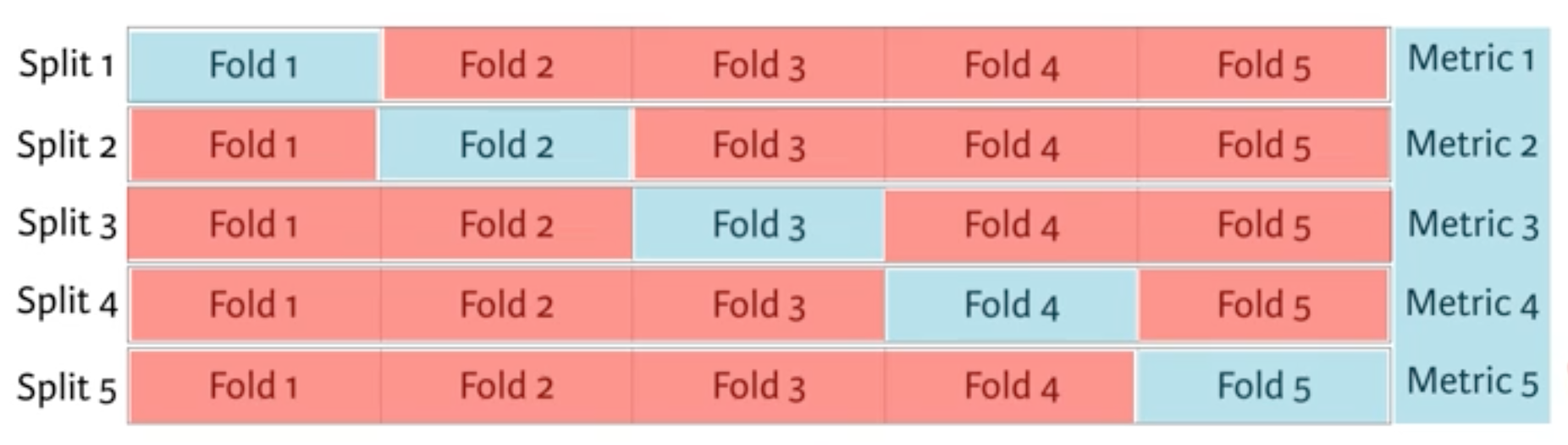
Split the dataset into 5 groups or folds. Then we hold out the first fold as a test set, fit the model on the remaining four folds, predict on the test set and compute the metric of interest. Next, we hold out the second fold as the test set, fit on the remaining data, predict on the test set and compute the metric of interest. Then similarly with the third, fourth and fifth.
As a result, we get five values of accuracy, from which we can compute statistics of interest, such as the median and/or mean and 95% confidence intervals.
We do this for each value of each hyperparameter that we are tuning and choose the set of hyperparameters that performs the best. This is called grid search.
In the following, we will use cross validation and grid search to choose the best max_depth for the new feature-engineered dataset:
# Setup the hyperparameter grid
dep = np.arange(1,9)
param_grid = {'max_depth' : dep}

# Instantiate a decision tree classifier: clf
clf = tree.DecisionTreeClassifier()

# Instantiate the GridSearchCV object: clf_cv
clf_cv = GridSearchCV(clf, param_grid=param_grid, cv=5)

# Fit it to the data
clf_cv.fit(X, y)

# Print the tuned parameter and score
print("Tuned Decision Tree Parameters: {}".format(clf_cv.best_params_))
print("Best score is {}".format(clf_cv.best_score_))
1 2 | |
Make predictions on the test set, create a new column Survived and store the predictions in it.
Save the PassengerId and Survived columns of df_test to a .csv and submit it to Kaggle.
Y_pred = clf_cv.predict(test)
df_test['Survived'] = Y_pred
df_test[['PassengerId', 'Survived']].to_csv('results/dec_tree_feat_eng.csv', index=False)
Submit to Kaggle (4th)
- Go to Kaggle, log in, and search for Titanic: Machine Learning from Disaster.
- Join the competition and submit the .csv file.
- Add a description and submit.
- Kaggle returns a ranking.
- At the time of the first submission: score 0.78468 (from 0.77980), rank 4009 (a jump of 819 places).