Importing Data
Foreword
Code snippets and excerpts from the courses. Python 3. From DataCamp.
Importing from Flat Files
- Load the script and run it.
# %load "Importing Data in Python.py"
file = open('moby_dick.txt', 'r')

# Print it
print(file.read())

# Check whether file is closed
print(file.closed)

# Close file
file.close()

# Check whether file is closed
print(file.closed)
1 2 3 4 5 6 7 8 9 10 11 12 13 14 15 16 17 18 19 20 | |
# Read & print the first 3 lines
with open('moby_dick.txt') as file:
    print(file.readline())
    print(file.readline())
    print(file.readline())
    print(file.readline(10))
    print(file.readline(50))
    print(file.readline(50))
1 2 3 4 5 6 7 | |
thisis a special package about PEP 20.
import this
1 2 3 4 5 6 7 8 9 10 11 12 13 14 15 16 17 18 19 20 21 | |
- BDFL: Benevolent Dictator For Life, a.k.a. Guido van Rossum, Python’s creator.
Numpy
- Numpy arrays are a standard for storing numerical data.
- Arrays are essential to other packages such as the
scikit-learn, for machine learning. - Import
numpyandmatplotlib(or invoke them with the%pylabmagic command).
import numpy as np
import matplotlib.pyplot as plt
# or...
%pylab inline

# no need for preceeding functions (methods) with np. or plt.
1 | |
- Import a csv file and assign the content to an array.
file = 'digits.csv'

# Load the file as an array called digits
digits = loadtxt(file, delimiter = ',')

# Print the datatype of digits
print(type(digits))

print(digits)

# Select a row
im = digits[2, 2:]
print(im)
1 2 3 4 5 6 7 8 | |
- Import a txt file. The
delimitercan be'\t',',',';', etc. - Skip the first 90 rows.
file = 'digits_header.txt'

# Load the data into array data
data = loadtxt(file, delimiter='  ', skiprows = 90)

# Print data
print(data)
1 2 3 4 5 6 7 8 9 10 | |
- Import a txt file, but only the last rows and first column.
data2 = loadtxt(file, delimiter='  ', skiprows = 90, usecols = [0])

# Print data
print(data2)
1 | |
- Import a txt file as string.
file = 'seaslug.txt'

# Import file: data
data = loadtxt(file, delimiter = ' ', dtype = str)

# Print the first element of data
print(data[0])
1 | |
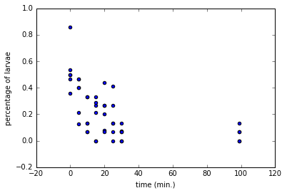
- Import a txt file as float numbers.
file = 'seaslug2.txt'

# Import data as floats and skip the first row: data_float
data_float = loadtxt(file, delimiter='   ', dtype = float, skiprows = 1)

# Print the 10th element of data_float
print(data_float[9])

# Plot a scatterplot of the data
scatter(data_float[:, 0], data_float[:, 1])
xlabel('time (min.)')
ylabel('percentage of larvae')

show()
1 | |
- Import a csv file. Format the data.
data = genfromtxt('titanic.csv', delimiter = ',', names = True, dtype = None)
 # A structred array
shape(data)
1 | |
- Extract a row, a column.
# to get the ith row, merely execute data[i]
print(data[0:10])
1 2 3 4 5 6 7 8 9 10 | |
# to get the column with name 'Fare', execute data['Fare']
print(data['Fare'][0:10])
1 2 | |
- Import a csv file.
- Format the data.
# default dtype is None
data2 = recfromcsv('titanic.csv', delimiter = ',', names = True, dtype = None)
# Print out first three entries
print(data2[:3])
1 2 3 | |
Pandas
- Two-dimensional labeled data structure(s) or data frame (DataFrame).
- Pythonic analog of R’s dataframes.
- Columns can be of potentially different types.
- Excellent object for:
- Manipulate, slice, reshape, groupby, join, merge.
- Perform statistics.
- Work with time series data.
- Exploratory data analysis.
- Data wrangling.
- Data preprocessing.
- Building models.
- Visualization.
- There exists standards and best practices to use Pandas.
# Import pandas
import pandas as pd
- Pandas is not part of
%pylab. - Import a file.
file = 'titanic.csv'

# Read the file into a DataFrame: df
df = pd.read_csv(file)

# View the head of the DataFrame
print(df.head())
1 2 3 4 5 6 7 8 9 10 11 12 13 | |
- Import another file; no header and some rows.
file = 'digits2.csv'

# Read the first 5 rows of the file into a DataFrame: data
data = pd.read_csv(file, nrows = 5, header = None)

# Print the datatype of data
print(type(data))

# Build a numpy array from the DataFrame: data_array
data_array = data.values

# Print the datatype of data_array to the shell
print(type(data_array))
1 2 | |
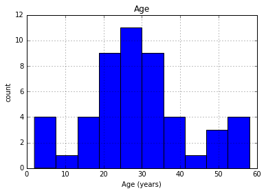
- Import another file; replace the missing data (NA).
file = 'titanic_corrupt.csv'

# Assign filename: file
file = 'titanic_corrupt.csv'

# Import file: data
data = pd.read_csv(file, sep = ';', comment = '#', na_values = ['Nothing'])

# Print the head of the DataFrame
print(data.head())
1 2 3 4 5 6 7 8 9 10 11 12 13 | |
- Plot the
Agevariable in a histogram.
pd.DataFrame.hist(data[['Age']])
plt.xlabel('Age (years)')
plt.ylabel('count')

plt.show()
Importing from Other Files
- With Pandas… and a bit of Numpy.
- Excel spreadsheets.
- MATLAB files.
- SAS files.
- Stata files.
- HDF5 files (large datasets, scientific, legal, etc.).
- Feather.
- Julia.
- Pickle files (binary).
import os

wd = os.getcwd()
os.listdir(wd)
1 2 3 4 5 6 7 8 9 10 11 12 13 14 15 16 17 18 19 20 21 22 23 24 25 26 27 28 29 30 31 32 33 34 35 36 37 38 39 40 41 42 43 44 45 46 | |
Pickled files
- There are a number of datatypes that cannot be saved easily to flat files, such as lists and dictionaries.
- If you want your files to be human readable, you may want to save them as text files in a clever manner (JSONs, which you will see in a later chapter, are appropriate for Python dictionaries).
- If, however, you merely want to be able to import them into Python, you can serialize them.
- All this means is converting the object into a sequence of bytes, or bytestream.
- Import it.
import pickle

# Save a dictionary into a pickle file.
fav = {'Airline' : '8', 'Aug' : '85', 'June' : '69.4', 'Mar' : '84.4'}
pickle.dump(fav, open("save.p", "wb"))

# save.p

# Open pickle file and load data: d

with open('save.p', 'rb') as file:
    d = pickle.load(file)

# Print d
print(d)

# Print datatype of d
print(type(d))
1 2 | |
Excel files
file = 'PRIO_bd3.0.xls'

# Load spreadsheet: xl
xl = pd.ExcelFile(file)

# Print sheet names
print(xl.sheet_names)
1 | |
- Parse the sheets.
- By name or by number (first, second, …).
df1 = xl.parse('bdonly')
df2 = xl.parse(0)
- Options: parse the first sheet by index, skip the first row of data, then name the columns
CountryandAAM due to War (2002).
df2 = xl.parse(0, parse_cols = [0], skiprows = [0], names = ['Country', 'AAM due to War (2002)'])
- Options: parse the second sheet, parse only the first column, skip the first row and rename the column
Country.
df2 = xl.parse(1, parse_cols = [0], skiprows = [0], names = ['Country'])
- Print the head of the
DataFrame.
print(df1.head())
1 2 3 4 5 6 7 8 9 10 11 12 13 14 15 16 17 18 19 20 21 22 | |
- We process images since we cheat a little.
- Many packages are not installed.
- We are not be able to import some data.
- Images will then present the final results.
from IPython.display import Image
# for the following pictures...
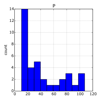
SAS files
- Advanced analytics
- Multivariate analysis
- Business intelligence
- Data management
- Predictive analytics
- Standard for computational analysis
- Code (instead of importing the package):
# Import sas7bdat package
from sas7bdat import SAS7BDAT

# Save file to a DataFrame: df_sas
with SAS7BDAT('sales.sas7bdat') as file:
    df_sas = file.to_data_frame()

# Print head of DataFrame
print(df_sas.head())

# Plot histogram of DataFrame features
pd.DataFrame.hist(df_sas[['P']])
plt.ylabel('count')

plt.show()
- The data are adapted from the website of the undergraduate text book Principles of Economics by Hill, Griffiths and Lim.
- The chart would be:
Image('p.png')
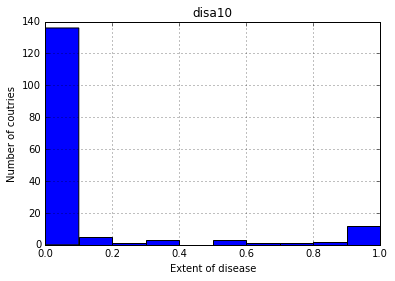
Stata files
- The data consist of disease extent for several diseases in various countries (more information can be found.
# Import pandas
import pandas as pd

# Load Stata file into a pandas DataFrame: df
df = pd.read_stata('disarea.dta')

# Print the head of the DataFrame df
print(df.head())
1 2 3 4 5 6 7 8 9 10 11 12 13 14 15 16 17 18 19 20 21 22 | |
- Plot histogram of one column of the
DataFrame.
pd.DataFrame.hist(df[['disa10']])
plt.xlabel('Extent of disease')
plt.ylabel('Number of coutries')

plt.show()
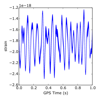
HDF5 files
- Standard for storing large quantities of numerical data.
- Datasets can be hundreds of gigabytes or terabytes.
- HDF5 can scale to exabytes.
- Code (instead of importing the package):
# Import packages
import numpy as np
import h5py

# Assign filename: file
file = 'LIGO_data.hdf5'

# Load file: data
data = h5py.File(file, 'r')

# Print the datatype of the loaded file
print(type(data))

# Print the keys of the file
for key in data.keys():
    print(key)

# Get the HDF5 group: group
group = data['strain']

# Check out keys of group
for key in group.keys():
    print(key)

# Set variable equal to time series data: strain
strain = data['strain']['Strain'].value

# Set number of time points to sample: num_samples
num_samples = 10000

# Set time vector
time = np.arange(0, 1, 1/num_samples)

# Plot data
plt.plot(time, strain[:num_samples])
plt.xlabel('GPS Time (s)')
plt.ylabel('strain')
plt.show()
- You can find the LIGO data plus loads of documentation and tutorials on Signal Processing with the data.
Image('strain.png')
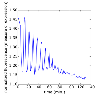
MATLAB
- “Matrix Laboratory”.
- Industry standard in engineering and science.
- Code (instead of importing the package):
# Import package
import scipy.io

# Load MATLAB file: mat
mat = scipy.io.loadmat('albeck_gene_expression.mat')

# Print the datatype type of mat
print(type(mat))

# Print the keys of the MATLAB dictionary
print(mat.keys())

# Print the type of the value corresponding to the key 'CYratioCyt'
print(type(mat['CYratioCyt']))

# Print the shape of the value corresponding to the key 'CYratioCyt'
print(np.shape(mat['CYratioCyt']))

# Subset the array and plot it
data = mat['CYratioCyt'][25, 5:]
fig = plt.figure()
plt.plot(data)
plt.xlabel('time (min.)')
plt.ylabel('normalized fluorescence (measure of expression)')
plt.show()
- This file contains gene expression data from the Albeck Lab at UC Davis. You can find the data and some great documentation.
Image('CYratioCyt.png')
Working with Relational Databases
Relational Database Management System
- PostgreSQL.
- MySQL.
- SQLite.
- Code (instead of importing the package):
# Import necessary module
from sqlalchemy import create_engine

# Create engine: engine
engine = create_engine('sqlite:///Chinook.sqlite')
'sqlite:///Northwind.sqlite' is called the connection string to the SQLite database.
- The Chinook database contains information about a semi-fictional digital media store in which media data is real and customer, employee and sales data has been manually created.
- Code (instead of importing the package):
# Save the table names to a list: table_names
table_names = engine.table_names()

# Print the table names to the shell
print(table_names)
Query the DB
- The final
;is facultative. - Code (instead of importing the package):
# Create engine: engine
engine = create_engine('sqlite:///Chinook.sqlite')

# Open engine connection: con
con = engine.connect()

# Perform query: rs
rs = con.execute('SELECT * FROM Album')

# Save results of the query to DataFrame: df
df = pd.DataFrame(rs.fetchall())

# Close connection
con.close()

# Print head of DataFrame df
print(df.head())
Customize queries
- Code (instead of importing the package):
# Create engine: engine
engine = create_engine('sqlite:///Chinook.sqlite') # becomes facultative with many queries

# Open engine in context manager
# Perform query and save results to DataFrame: df
with engine.connect() as con:
    rs = con.execute('SELECT LastName, Title FROM Employee')
    df = pd.DataFrame(rs.fetchmany(size = 3))
    df.columns = rs.keys() # set the DataFrame's column names to the corresponding names of the table columns

# Print the length of the DataFrame df
print(len(df))

# Print the head of the DataFrame df
print(df.head())
- Code (instead of importing the package):
# Create engine: engine
engine = create_engine('sqlite:///Chinook.sqlite') # becomes facultative with many queries

# Open engine in context manager
# Perform query and save results to DataFrame: df
with engine.connect() as con:
    rs = con.execute("SELECT * FROM Employee WHERE EmployeeId >= 6")
    df = pd.DataFrame(rs.fetchall())
    df.columns = rs.keys()

# Print the head of the DataFrame df
print(df.head())
- Code (instead of importing the package):
# Create engine: engine
engine = create_engine('sqlite:///Chinook.sqlite')

# Open engine in context manager
with engine.connect() as con:
    rs = con.execute('SELECT * FROM Employee ORDER BY BirthDate')
    df = pd.DataFrame(rs.fetchall())

    # Set the DataFrame's column names
    df.columns = rs.keys()

# Print head of DataFrame
print(df.head())
Query the DB the Pandas way
- Simpler code (instead of importing the package)!!!
# Import packages
from sqlalchemy import create_engine
import pandas as pd

# Create engine: engine
engine = create_engine('sqlite:///Chinook.sqlite')

# Execute query and store records in DataFrame: df
df = pd.read_sql_query("SELECT * FROM Album", engine)

# Print head of DataFrame
print(df.head())

# Open engine in context manager
# Perform query and save results to DataFrame: df1
with engine.connect() as con:
    rs = con.execute("SELECT * FROM Album")
    df1 = pd.DataFrame(rs.fetchall())
    df1.columns = rs.keys()

# Confirm that both methods yield the same result: does df = df1 ?
print(df.equals(df1))
- Code (instead of importing the package):
# Import packages
from sqlalchemy import create_engine
import pandas as pd

# Create engine: engine
engine = create_engine('sqlite:///Chinook.sqlite')

# Execute query and store records in DataFrame: df
df = pd.read_sql_query("SELECT * FROM Employee WHERE EmployeeId >= 6 ORDER BY BirthDate", engine)

# Print head of DataFrame
print(df.head())
INNER JOIN
- Code (instead of importing the package):
import pandas as pd
from sqlalchemy import create_engine

engine = create_engine('sqlite:///Chinook.sqlite')

# Open engine in context manager
# Perform query and save results to DataFrame: df
with engine.connect() as con:
    rs = con.execute("SELECT Title, Name FROM Album INNER JOIN Artist on Album.ArtistID = Artist.ArtistID")
    df = pd.DataFrame(rs.fetchall())
    df.columns = rs.keys()

# Print head of DataFrame df
print(df.head())
- Alternative code:
df = pd.read_sql_query("SELECT Title, Name FROM Album INNER JOIN Artist on Album.ArtistID = Artist.ArtistID", engine)

# Print head of DataFrame df
print(df.head())
- Code (instead of importing the package):
# Execute query and store records in DataFrame: df
df = pd.read_sql_query("SELECT * FROM PlaylistTrack INNER JOIN Track on PlaylistTrack.TrackId = Track.TrackId WHERE Milliseconds < 250000", engine)

# Print head of DataFrame
print(df.head())
Importing Flat Files from the Web (Web Scraping)
- Import and locally save datasets from the web.
- Load datasets into Pandas
DataFrame. - Make HTTP requests (GET requests).
- Scrape web data such as HTML.
- Parse HTML into useful data (BeautifulSoup).
- Use the urllib and requests packages.
Using the urllib package on csv files
- Import the package.
from urllib.request import urlretrieve

# import pandas as pd

# Assign url of file: url
url = 'http://archive.ics.uci.edu/ml/machine-learning-databases/wine-quality/winequality-red.csv'

# Save file locally
urlretrieve(url, 'winequality-red.csv')

# Read file into a DataFrame and print its head
df = pd.read_csv('winequality-red.csv', sep=';')
print(df.head())
1 2 3 4 5 6 7 8 9 10 11 12 13 14 15 16 17 18 19 20 | |
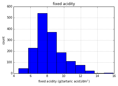
# import matplotlib.pyplot as plt
# import pandas as pd

# Assign url of file: url
url = 'http://archive.ics.uci.edu/ml/machine-learning-databases/wine-quality/winequality-red.csv'

# Read file into a DataFrame: df
df = pd.read_csv(url, sep = ';')

# Print the head of the DataFrame
print(df.head())

# Plot first column of df
pd.DataFrame.hist(df.ix[:, 0:1])
plt.xlabel('fixed acidity (g(tartaric acid)/dm$^3$)')
plt.ylabel('count')
plt.show()
1 2 3 4 5 6 7 8 9 10 11 12 13 14 15 16 17 18 19 20 | |
Using the urllib package on Excel files
# import pandas as pd

# Assign url of file: url
url = 'http://s3.amazonaws.com/assets.datacamp.com/course/importing_data_into_r/latitude.xls'

# Read in all sheets of Excel file: xl
xl = pd.read_excel(url, sheetname = None)

# Print the sheetnames (keys) to the shell !!!
print(xl.keys())

# Print the head of the first sheet (using its name, NOT its index)
print(xl['1700'].head())
1 2 3 4 5 6 7 | |
HTTP requests to import files from the web
requestsis one of the most downloaded Python packages.requestsworks withurllib.- Import the package.
from urllib.request import urlopen, Request

# Specify the url
url = "http://www.datacamp.com/teach/documentation"

# This packages the request: request
request = Request(url)

# Send the request and catches the response: response
response = urlopen(request)

# Print the datatype of response
print(type(response))

# Be polite and close the response!
response.close()
1 | |
from urllib.request import urlopen, Request

url = "http://docs.datacamp.com/teach/"

request = Request(url)

response = urlopen(request)


# Extract the response: html
html = response.read()

# Print the html
print(html)

# Be polite and close the response!
response.close()
1 | |
Using requests
import requests

url = "http://docs.datacamp.com/teach/"

r = requests.get(url)

text = r.text

# Print part of the html (split the paragraphs) instead of all with  print(text)
head = text.split('\n\n')

print(head[0])
print('')
print(head[1])
print('')
print(head[2])
print('')
print(head[3])
1 2 3 4 5 6 7 8 9 10 11 12 13 14 15 16 | |
Scraping the web
- Scrape unstructured data.
- Scrape structured data, parse it and extract the data from HTML using the BeautifulSoup package.
- Import the packages.
import requests
from bs4 import BeautifulSoup

url = 'https://www.python.org/~guido/'

r = requests.get(url)

html_doc = r.text

# Create a BeautifulSoup object from the HTML: soup
soup = BeautifulSoup(html_doc, 'lxml')

# Prettify the BeautifulSoup object: pretty_soup
pretty_soup = soup.prettify()

# Print the response
print(type(pretty_soup))

# Print part of the html (split the text), not all with  print(pretty_soup)
head = pretty_soup.split('</h3>')

print(head[0])
1 2 3 4 5 6 7 8 9 10 11 12 13 14 15 16 17 18 19 20 21 22 23 24 25 26 | |
- Other operations with BeautifulSoup.
import requests
from bs4 import BeautifulSoup

url = 'https://www.python.org/~guido/'

r = requests.get(url)

html_doc = r.text


# Create a BeautifulSoup object from the HTML: soup
soup = BeautifulSoup(html_doc, 'lxml')

# Get the title of Guido's webpage: guido_title
guido_title = soup.title # attribute

# Print the title of Guido's webpage to the shell
print(guido_title)

# Get Guido's text: guido_text
guido_text = soup.get_text() # method

# Print Guido's text to the shell
print(guido_text)
1 2 3 4 5 6 7 8 9 10 11 12 13 14 15 16 17 18 19 20 21 22 23 24 25 26 27 28 29 30 31 32 33 34 35 36 37 38 39 40 41 42 43 44 45 46 47 48 49 50 51 52 53 54 55 56 57 58 59 60 61 62 63 64 65 66 67 68 69 70 71 72 73 74 75 76 | |
- More.
import requests
from bs4 import BeautifulSoup

url = 'https://www.python.org/~guido/'

r = requests.get(url)

html_doc = r.text

# create a BeautifulSoup object from the HTML: soup
soup = BeautifulSoup(html_doc, 'lxml')

# Print the title of Guido's webpage
print(soup.title)

# Find all 'a' tags (which define hyperlinks): a_tags
a_tags = soup.find_all('a') # for <a>, hyperlinks

# Print the URLs to the shell
for link in a_tags:
    print( link.get('href'))
1 2 3 4 5 6 7 8 9 10 11 12 13 14 15 16 17 18 19 20 21 22 23 24 25 26 | |
Introduction to APIs and JSONs
- API or Application Programming Interface are protocols and routines providing access to websites and web apps like OMDb, Wikipedia, Uber, Uber Developers, BGG, ImDB, Facebook, Instagram, and Twitter.
- Most of data coming from APIS are JSON files.
Import the json package
import json

# Load JSON: json_data
with open('a_movie.json', 'r') as json_file:
    json_data = json.load(json_file)

print(type(json_data))
print(json_data['Title'])
print(json_data['Year'])
print('')

# Print each key-value pair in json_data
for k in json_data.keys():
    print(k + ': ', json_data[k])
1 2 3 4 5 6 7 8 9 10 11 12 13 14 15 16 17 18 19 20 21 22 23 24 | |
The requests package again
- Pull some movie data down from the Open Movie Database (OMDB) using their API.
- Pull it as text.
import requests

url = 'http://www.omdbapi.com/?t=social+network'

r = requests.get(url)

print(type(r))
print('')

# Print the text of the response
print(r.text)
1 2 3 | |
- Pull it as JSON or a dictionary.
import requests

url = 'http://www.omdbapi.com/?t=social+network'

r = requests.get(url)

# Decode the JSON data into a dictionary: json_data
json_data = r.json()

print(type(json_data))
print('')

# Print each key-value pair in json_data
for k in json_data.keys():
    print(k + ': ', json_data[k])
1 2 3 4 5 6 7 8 9 10 11 12 13 14 15 16 17 18 19 20 21 22 | |
- Search the Library of Congress.
- Pull a dictionary of dictionaries.
import requests

url = 'http://chroniclingamerica.loc.gov/search/titles/results/?terms=new%20york&format=json'

r = requests.get(url)

# Decode the JSON data into a dictionary: json_data
json_data = r.json()

# Select the first element in the list json_data['items']: nyc_loc
# dict of dict
nyc_loc = json_data['items'][0]

# Print each key-value pair in nyc_loc
for k in nyc_loc.keys():
    print(k + ': ', nyc_loc[k])
1 2 3 4 5 6 7 8 9 10 11 12 13 14 15 16 17 18 19 20 21 22 23 24 | |
- The Wikipedia API.
- Documentation.
- Dictionary of dictionary of dictionary.
import requests

url = 'https://en.wikipedia.org/w/api.php?action=query&prop=extracts&format=json&exintro=&titles=pizza'

r = requests.get(url)

# Decode the JSON data into a dictionary: json_data
json_data = r.json()

# Print the Wikipedia page extract
pizza_extract = json_data['query']['pages']['24768']['extract']
print(pizza_extract)
1 2 3 4 | |
The Twitter API and Authentification
- Twitter has many APIs: the main API, the REST API, Streaming APIs (private, public), Firehouse (expensive), etc.
- Field Guide.
- Consult the documentation to set an authentification key (available online).
tweepy package
- The authentication looks like the following:
- Code:
# Import package
import tweepy, json

# Store OAuth authentication credentials in relevant variables
access_token = "---"
access_token_secret = "---"
consumer_key = "---"
consumer_secret = "---"

# Pass OAuth details to tweepy's OAuth handler
auth = tweepy.OAuthHandler(consumer_key, consumer_secret)
auth.set_access_token(access_token, access_token_secret)
Start streaming tweets
- Code:
# Initialize Stream listener
l = MyStreamListener()

# Create you Stream object with authentication
stream = tweepy.Stream(auth, l)


# Filter Twitter Streams to capture data by the keywords:
stream.filter(track = ['clinton', 'trump', 'sanders', 'cruz'])
- Code of
MyStreamListener(): - Creates a file called tweets.txt, collects streaming tweets as .jsons and writes them to the file tweets.txt; once 100 tweets have been streamed, the listener closes the file and stops listening.
class MyStreamListener(tweepy.StreamListener):


    def __init__(self, api=None):

        super(MyStreamListener, self).__init__()
        self.num_tweets = 0
        self.file = open("tweets.txt", "w")

    def on_status(self, status):

        tweet = status._json
        self.file.write( json.dumps(tweet) + '\n' )
        tweet_list.append(status)
        self.num_tweets += 1
        if self.num_tweets < 100:
            return True
        else:
            return False
        self.file.close()

    def on_error(self, status):
        print(status)
Load and explore your Twitter data
- Code:
# Import package
import json

# String of path to file: tweets_data_path
tweets_data_path = 'tweets.txt'

# Initialize empty list to store tweets: tweets_data
tweets_data = []

# Open connection to file
tweets_file = open(tweets_data_path, "r")

# Read in tweets and store in list: tweets_data
for line in tweets_file:
    tweet = json.loads(line)
    tweets_data.append(tweet)

# Close connection to file
tweets_file.close()

# Print the keys of the first tweet dict
print(tweets_data[0].keys())
Send the Twitter data to a DataFrame
- Twitter data in a list of dictionaries
tweets_data, where each dictionary corresponds to a single tweet. - The text in a tweet
t1is stored as the valuet1['text']; similarly, the language is stored int1['lang']. - Code:
# Import package
import pandas as pd

# Build DataFrame of tweet texts and languages
df = pd.DataFrame(tweets_data, columns=['text', 'lang'])

# Print head of DataFrame
print(df.head())
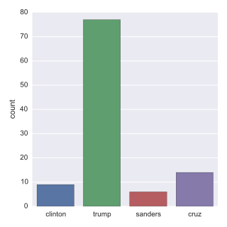
Analyze the tweets (NLP, regex)
- A little bit of Twitter text analysis and plotting.
- Use the statistical data visualization library seaborn.
- Code:
# Import the regular expressions library
import re

# The function tells you whether the first argument (a word) occurs within the 2nd argument (a tweet)
def word_in_text(word, tweet):
    word = word.lower()
    text = tweet.lower()
    match = re.search(word, tweet)

    if match:
        return True
    return False

# Initialize list to store tweet counts
[clinton, trump, sanders, cruz] = [0, 0, 0, 0]

# Iterate through df, counting the number of tweets in which
# each candidate is mentioned
for index, row in df.iterrows():
    clinton += word_in_text('clinton', row['text'])
    trump += word_in_text('trump', row['text'])
    sanders += word_in_text('sanders', row['text'])
    cruz += word_in_text('cruz', row['text'])

# Import packages
import matplotlib.pyplot as plt
import seaborn as sns

# Set seaborn style
sns.set(color_codes=True)

# Create a list of labels:cd
cd = ['clinton', 'trump', 'sanders', 'cruz']

# Plot histogram
ax = sns.barplot(cd, [clinton, trump, sanders, cruz])
ax.set(ylabel="count")
plt.show()
from IPython.display import Image
# for the following pictures...
Image('tweets_figure.png')