%pylabinlineimportpandasaspd# Import Times Higher Education World University Rankings data# https://www.timeshighereducation.com/world-university-rankingstimes_df=pd.read_csv('timesData.csv',thousands=",")# Import Academic Ranking of World Universities data# http://www.shanghairanking.com/shanghai_df=pd.read_csv('shanghaiData.csv')
1
Populating the interactive namespace from numpy and matplotlib
# Retrieve the values at columns and rows 1-3print(times_df.iloc[1:4,1:4])
1234
                         university_name                   country  teaching
1     California Institute of Technology  United States of America      97.7
2  Massachusetts Institute of Technology  United States of America      97.8
3                    Stanford University  United States of America      98.3
# Retrieve the column `total_score`
print(times_df['total_score'])
# Query `shanghai_df` for universities with total score between 40 and 50average_schools=shanghai_df.query('total_score > 0 and total_score < 50')# Print the resultprint(average_schools)
pipe() to chain operations and thus eliminate the need for intermediate DataFrames.
Without this operator, instead of writing df.pipe(f).pipe(g).pipe(h) write: h(g(f(df))). This becomes harder to follow once the number of nested functions grows large.
# Clean up the `world_rank` defclean_world_rank(input_df):df=input_df.copy()df.world_rank=df.world_rank.str.split('-').str[0].str.split('=').str[0]returndf
# Assign the common years of `shanghai_df` and `times_df` to `common_years` common_years=set(shanghai_df.year)&set(times_df.year)# Print `common_years`print(common_years)
1
{2011, 2012, 2013, 2014, 2015}
# Filter yearsdeffilter_year(input_df,years):df=input_df.copy()returndf.query('year in {}'.format(list(years)))
# Clean `times_df` and `shanghai_df`cleaned_times_df=(times_df.loc[:,common_columns].pipe(filter_year,common_years).pipe(clean_world_rank).assign(name='times'))cleaned_shanghai_df=(shanghai_df.loc[:,common_columns].pipe(filter_year,common_years).pipe(clean_world_rank).assign(name='shanghai'))
38% of data missing from the total_score column: drop this column with the .drop method.
# Compose `ranking_df` with `cleaned_times_df` and `cleaned_shanghai_df`ranking_df=pd.concat([cleaned_times_df,cleaned_shanghai_df])# Calculate the percentage of missing datamissing_data=100*pd.isnull(ranking_df.total_score).sum()/len(ranking_df)# Drop the `total_score` column of `ranking_df`ranking_df=ranking_df.drop('total_score',axis=1)
Memory can start to play a big part in how fast the pipelines can run. Without the “deep” flag turned on, Pandas won’t estimate memory consumption for the object dtype: category when dealing with categorical data, etc. int64 or even int16 takes less memory.
# Print the memory usage of `ranking_df`
ranking_df.info()
123456789
<class 'pandas.core.frame.DataFrame'>
Int64Index: 3686 entries, 0 to 4896
Data columns (total 4 columns):
year               3686 non-null int64
world_rank         3686 non-null object
university_name    3685 non-null object
name               3686 non-null object
dtypes: int64(1), object(3)
memory usage: 144.0+ KB
# Print the deep memory usage of `ranking_df`
ranking_df.info(memory_usage="deep")
123456789
<class 'pandas.core.frame.DataFrame'>
Int64Index: 3686 entries, 0 to 4896
Data columns (total 4 columns):
year               3686 non-null int64
world_rank         3686 non-null object
university_name    3685 non-null object
name               3686 non-null object
dtypes: int64(1), object(3)
memory usage: 803.1 KB
defmemory_change(input_df,column,dtype):df=input_df.copy()old=round(df[column].memory_usage(deep=True)/1024,2)# In KBnew=round(df[column].astype(dtype).memory_usage(deep=True)/1024,2)# In KBchange=round(100*(old-new)/(old),2)report=("The inital memory footprint for {column} is: {old}KB.\n""The casted {column} now takes: {new}KB.\n""A change of {change} %.").format(**locals())returnreport
‘Massachusetts Institute of Technology (MIT)’ and ‘Massachusetts Institute of Technology’ are two different records of the same university. Thus, change the first name to the latter.
# Query for the rows with university name 'Massachusetts Institute of Technology (MIT)'print(ranking_df.query("university_name == 'Massachusetts Institute of Technology (MIT)'"))
123456
      year                              university_name  world_rank      name
3016  2011  Massachusetts Institute of Technology (MIT)           3  shanghai
3516  2012  Massachusetts Institute of Technology (MIT)           3  shanghai
3801  2013  Massachusetts Institute of Technology (MIT)           4  shanghai
3899  2014  Massachusetts Institute of Technology (MIT)           3  shanghai
4399  2015  Massachusetts Institute of Technology (MIT)           3  shanghai
ranking_df.loc[ranking_df.university_name=='Massachusetts Institute of Technology (MIT)','university_name']='Massachusetts Institute of Technology'
To find the 5 (more generally n) top universities over the years, for each ranking system, here is how to do it in pseudo-code:
For each year (in the year column) and for each ranking system (in the name column):
Select the subset of the data for this given year and the given ranking system.
Select the 5 top universities and store them in a list.
Store the result in a dictionary with (year, name) as key and the list of the universities (in descending order) as the value.
# Load in `itertools`importitertools# Initialize `ranking`ranking={}foryear,nameinitertools.product(common_years,["times","shanghai"]):s=(ranking_df.loc[lambdadf:((df.year==year)&(df.name==name)&(df.world_rank.isin(range(1,6)))),:].sort_values('world_rank',ascending=False).university_name)ranking[(year,name)]=list(s)# Print `ranking`print(ranking)
1
{(2011,'times'):['Princeton University','Stanford University','Massachusetts Institute of Technology','California Institute of Technology','Harvard University'],(2011,'shanghai'):['University of Cambridge','University of California, Berkeley','Massachusetts Institute of Technology','Stanford University','Harvard University'],(2012,'times'):['Princeton University','University of Oxford','Harvard University','Stanford University','California Institute of Technology'],(2012,'shanghai'):['University of Cambridge','University of California, Berkeley','Massachusetts Institute of Technology','Stanford University','Harvard University'],(2013,'times'):['Massachusetts Institute of Technology','Harvard University','Stanford University','University of Oxford','California Institute of Technology'],(2013,'shanghai'):['University of Cambridge','Massachusetts Institute of Technology','University of California, Berkeley','Stanford University','Harvard University'],(2014,'times'):['Massachusetts Institute of Technology','Stanford University','Harvard University','University of Oxford','California Institute of Technology'],(2014,'shanghai'):['University of Cambridge','University of California-Berkeley','Massachusetts Institute of Technology','Stanford University','Harvard University'],(2015,'times'):['University of Cambridge','Stanford University','University of Oxford','Harvard University','California Institute of Technology'],(2015,'shanghai'):['University of Cambridge','University of California, Berkeley','Massachusetts Institute of Technology','Stanford University','Harvard University']}
We have this ranking dictionary, let’s find out how much (in percentage) both ranking methods differ over the years: the two are 100% set-similar if the selected 5-top universities are the same even though they aren’t ranked the same.
# Construct a DataFrame with the top 5 universities top_5_df=ranking_df.loc[lambdadf:df.world_rank.isin(range(1,6)),:]# Print the first rows of `top_5_df`top_5_df.head()
year
university_name
world_rank
name
0
2011
Harvard University
1
times
1
2011
California Institute of Technology
2
times
2
2011
Massachusetts Institute of Technology
3
times
3
2011
Stanford University
4
times
4
2011
Princeton University
5
times
top_5_df.tail()
year
university_name
world_rank
name
4397
2015
Harvard University
1
shanghai
4398
2015
Stanford University
2
shanghai
4399
2015
Massachusetts Institute of Technology
3
shanghai
4400
2015
University of California, Berkeley
4
shanghai
4401
2015
University of Cambridge
5
shanghai
# Compute the similaritydefcompute_set_similarity(s):pivoted=s.pivot(values='world_rank',columns='name',index='university_name').dropna()set_simlarity=100*len((set(pivoted['shanghai'].index)&set(pivoted['times'].index)))/5returnset_simlarity# Group `top_5_df` by `year` grouped_df=top_5_df.groupby('year')# Use `compute_set_similarity` to construct a DataFramesetsimilarity_df=pd.DataFrame({'set_similarity':grouped_df.apply(compute_set_similarity)}).reset_index()# Print the first rows of `setsimilarity_df`setsimilarity_df.head()
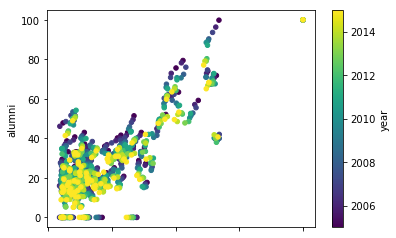
There are some 0 values for the alumni column (0, -, NaN, etc.). Remove them.
# Replace `-` entries with NaN valuestimes_df['total_score']=times_df['total_score'].replace("-","NaN").astype('float')# Drop all rows with NaN values for `num_students` times_df=times_df.dropna(subset=['num_students'],how='all')# Cast the remaining rows with `num_students` as inttimes_df['num_students']=times_df['num_students'].astype('int')
# Plot a scatterplot with `total_score` and `num_students`times_df.plot.scatter('total_score','num_students',c='year',colormap='viridis')plt.show()
The Seaborn plotting tool is mainly used to create statistical plots that are visually appealing.
importseabornassns# Set the Seaborn theme if desiredsns.set_style('darkgrid')
# Abbreviate country names of United States and United Kingdomtimes_df['country']=times_df['country'].replace("United States of America","USA").replace("United Kingdom","UK")# Count the frequency of countries count=times_df['country'].value_counts()[:10]# Convert the top 10 countries to a DataFrame df=count.to_frame()
# Reset the index #df.reset_index(level=0, inplace=True)# or...df['index1']=df.indexdf
country
index1
USA
625
USA
UK
286
UK
Germany
150
Germany
Australia
117
Australia
Canada
108
Canada
Japan
98
Japan
Italy
94
Italy
China
82
China
Netherlands
75
Netherlands
France
73
France
# Rename the columnsdf.columns=['count','country',]
# Plot a barplot with `country` and `count`sns.barplot(x='country',y='count',data=df)sns.despine()plt.show()
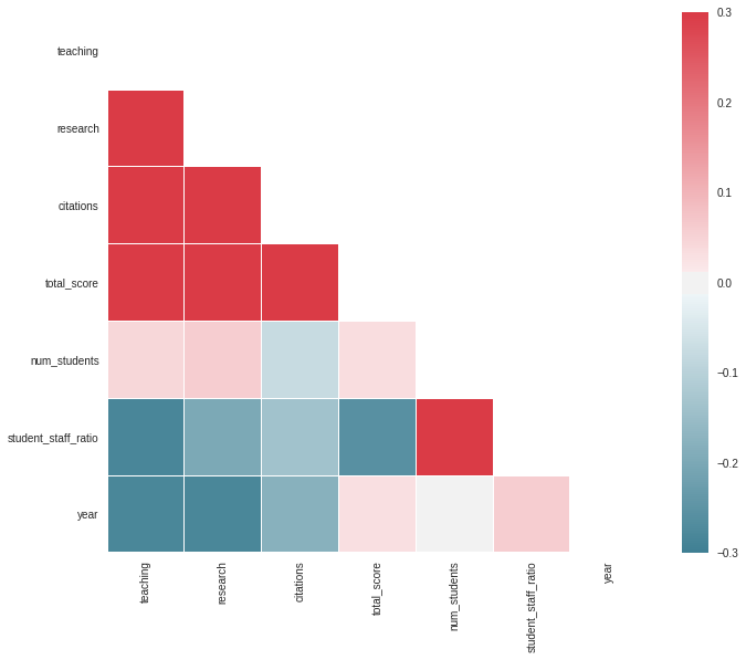
sns.set(style="white")# Compute the correlation matrixcorr=times_df.corr()# Generate a mask for the upper trianglemask=np.zeros_like(corr,dtype=np.bool)mask[np.triu_indices_from(mask)]=True# Set up the matplotlib figuref,ax=plt.subplots(figsize=(11,9))# Generate a custom diverging colormapcmap=sns.diverging_palette(220,10,as_cmap=True)# Draw the heatmap with the mask and correct aspect ratiosns.heatmap(corr,mask=mask,cmap=cmap,vmax=.3,square=True,linewidths=.5,ax=ax)plt.show()