# Take a quick peek at both vectorsA<-PE$activeyearsB<-PE$endurance# Save the differences of each vector element with the mean in a new variablediff_A<-A-mean(A)diff_B<-B-mean(B)# Do the summation of the elements of the vectors and divide by N-1 in order to acquire the covariance between the two vectorscov<-sum(diff_A*diff_B)/(length(A)-1)cov
1
## [1] 16.59045
Manual computation of correlation coefficients - Part 2
# Square the differences that were found in the previous stepsq_diff_A<-diff_A^2sq_diff_B<-diff_B^2# Take the sum of the elements, divide them by N-1 and consequently take the square root to acquire the sample standard deviationssd_A<-sqrt(sum(sq_diff_A)/(length(A)-1))sd_B<-sqrt(sum(sq_diff_B)/(length(B)-1))sd_A
1
## [1] 4.687134
sd_B
1
## [1] 10.83963
Manual computation of correlation coefficients - part 3
# Combine all the pieces of the puzzlecorrelation<-cov/(sd_A*sd_B)correlation
1
## [1] 0.3265402
# Check the validity of your result with the cor() commandcor(A,B)
1
## [1] 0.3265402
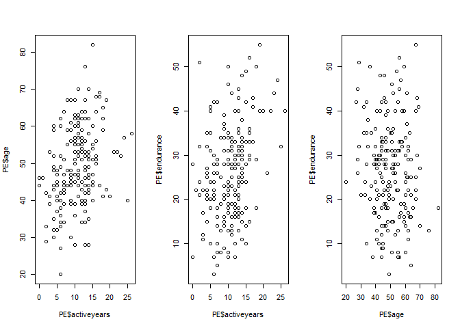
Creating scatterplots
library(psych)# Summary statisticsdescribe(PE)
1 2 3 4 5 6 7 8 910
## vars n mean sd median trimmed mad min max range skew## pid 1 200 101.81 58.85 101.5 101.71 74.87 1 204 203 0.01## age 2 200 49.41 10.48 48.0 49.46 10.38 20 82 62 0.06## activeyears 3 200 10.68 4.69 11.0 10.57 4.45 0 26 26 0.30## endurance 4 200 26.50 10.84 27.0 26.22 10.38 3 55 52 0.22## kurtosis se## pid -1.21 4.16## age -0.14 0.74## activeyears 0.46 0.33## endurance -0.44 0.77
## age activeyears endurance
## age 1.00 0.33 -0.08
## activeyears 0.33 1.00 0.33
## endurance -0.08 0.33 1.00
# Do some correlation tests. If the null hypothesis of no correlation can be rejected on a significance level of 5%, then the relationship between variables is significantly different from zero at the 95% confidence levelcor.test(PE$age,PE$activeyears)
1 2 3 4 5 6 7 8 91011
##
##  Pearson's product-moment correlation
##
## data:  PE$age and PE$activeyears
## t = 4.9022, df = 198, p-value = 1.969e-06
## alternative hypothesis: true correlation is not equal to 0
## 95 percent confidence interval:
##  0.1993491 0.4473145
## sample estimates:
##       cor
## 0.3289909
cor.test(PE$age,PE$endurance)
1 2 3 4 5 6 7 8 91011
##
##  Pearson's product-moment correlation
##
## data:  PE$age and PE$endurance
## t = -1.1981, df = 198, p-value = 0.2323
## alternative hypothesis: true correlation is not equal to 0
## 95 percent confidence interval:
##  -0.22097811  0.05454491
## sample estimates:
##         cor
## -0.08483813
cor.test(PE$endurance,PE$activeyears)
1 2 3 4 5 6 7 8 91011
##
##  Pearson's product-moment correlation
##
## data:  PE$endurance and PE$activeyears
## t = 4.8613, df = 198, p-value = 2.37e-06
## alternative hypothesis: true correlation is not equal to 0
## 95 percent confidence interval:
##  0.1967110 0.4451154
## sample estimates:
##       cor
## 0.3265402
CAUTION:
The magnitude of a correlation depends upon many factors, including sampling.
The magnitude of a correlation is also influenced by measurement of X & Y.
The correlation coefficient is a sample statistic, just like the mean.
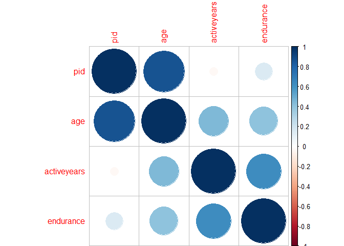
# Create a correlation matrix for the dataset (9-14 are the '2' variables only)correlations<-cor(PE[9:14,])# Create the scatterplot matrix for the datasetlibrary(corrplot)corrplot(correlations)
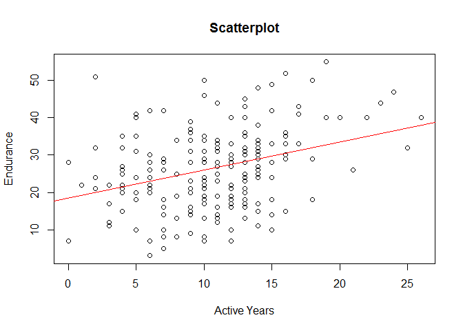
Manual computation of a simple linear regression
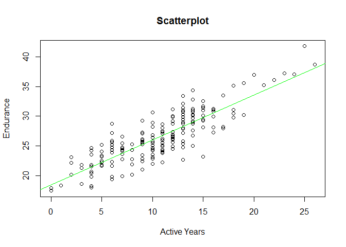
# Calculate the required means, standard deviations and correlation coefficientmean_ay<-mean(PE$activeyears)mean_e<-mean(PE$endurance)sd_ay<-sd(PE$activeyears)sd_e<-sd(PE$endurance)r<-cor(PE$activeyears,PE$endurance)# Calculate the slopeB_1<-r*(sd_e)/(sd_ay)# Calculate the interceptB_0<-mean_e-B_1*mean_ay# Plot of ic2 against sym2plot(PE$activeyear,PE$endurance,main='Scatterplot',ylab='Endurance',xlab='Active Years')# Add the regression lineabline(B_0,B_1,col='red')
Executing a simple linear regression using R
# Construct the regression modelmodel_1<-lm(PE$endurance~PE$activeyear)# Look at the results of the regression by using the summary functionsummary(model_1)
1 2 3 4 5 6 7 8 9101112131415161718
##
## Call:
## lm(formula = PE$endurance ~ PE$activeyear)
##
## Residuals:
##      Min       1Q   Median       3Q      Max
## -20.5006  -7.8066   0.5304   5.7649  31.0511
##
## Coefficients:
##               Estimate Std. Error t value Pr(>|t|)
## (Intercept)    18.4386     1.8104  10.185  < 2e-16 ***
## PE$activeyear   0.7552     0.1553   4.861 2.37e-06 ***
## ---
## Signif. codes:  0 '***' 0.001 '**' 0.01 '*' 0.05 '.' 0.1 ' ' 1
##
## Residual standard error: 10.27 on 198 degrees of freedom
## Multiple R-squared:  0.1066, Adjusted R-squared:  0.1021
## F-statistic: 23.63 on 1 and 198 DF,  p-value: 2.37e-06
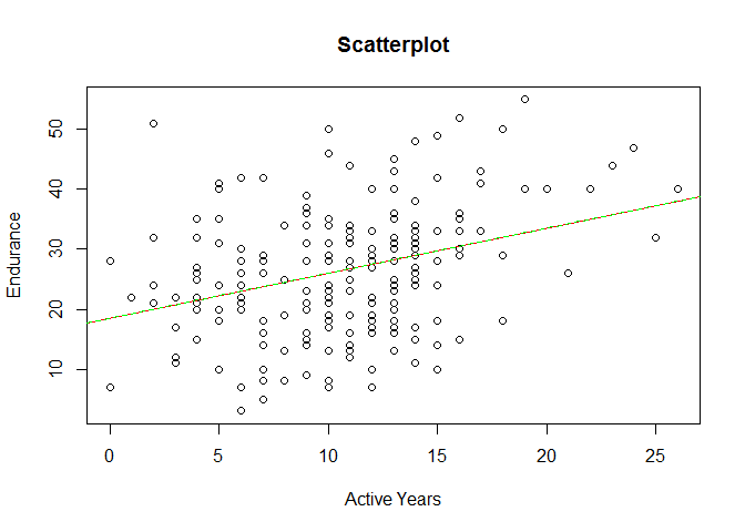
# Extract the predicted valuespredicted<-fitted(model_1)# Create a scatter plot of Impulse Control against Symptom Scoreplot(PE$endurance~PE$activeyear,main='Scatterplot',ylab='Endurance',xlab='Active Years')# Add a regression lineabline(model_1,col='red')abline(lm(predicted~PE$activeyears),col='green',lty=2)
Executing a multiple regression in R
# Multiple Regressionmodel_2<-lm(PE$endurance~PE$activeyear+PE$age)# Examine the results of the regressionsummary(model_2)
# Create a linear regression with `ic2` and `vismem2` as regressorsmodel_1<-lm(PE$endurance~PE$activeyear+PE$age)# Extract the predicted valuespredicted_1<-fitted(model_1)# Calculate the squared deviation of the predicted values from the observed values deviation_1<-(predicted_1-PE$endurance)^2# Sum the squared deviationsSSR_1<-sum(deviation_1)SSR_1
1
## [1] 19919.55
Standardized linear regression
# Create a standardized simple linear regressionmodel_1_z<-lm(scale(PE$endurance)~scale(PE$activeyear))# Look at the output of this regression modelsummary(model_1_z)
1 2 3 4 5 6 7 8 9101112131415161718
##
## Call:
## lm(formula = scale(PE$endurance) ~ scale(PE$activeyear))
##
## Residuals:
##      Min       1Q   Median       3Q      Max
## -1.89126 -0.72019  0.04893  0.53184  2.86459
##
## Coefficients:
##                       Estimate Std. Error t value Pr(>|t|)
## (Intercept)          4.871e-17  6.700e-02   0.000        1
## scale(PE$activeyear) 3.265e-01  6.717e-02   4.861 2.37e-06 ***
## ---
## Signif. codes:  0 '***' 0.001 '**' 0.01 '*' 0.05 '.' 0.1 ' ' 1
##
## Residual standard error: 0.9476 on 198 degrees of freedom
## Multiple R-squared:  0.1066, Adjusted R-squared:  0.1021
## F-statistic: 23.63 on 1 and 198 DF,  p-value: 2.37e-06
# Extract the R-Squared value for this regressionr_square_1<-summary(model_1_z)$r.squaredr_square_1
1
## [1] 0.1066285
# Calculate the correlation coefficientcorr_coef_1<-sqrt(r_square_1)corr_coef_1
1
## [1] 0.3265402
# Create a standardized multiple linear regressionmodel_2_z<-lm(scale(PE$endurance)~scale(PE$activeyear)+scale(PE$age))# Look at the output of this regression modelsummary(model_2_z)
# Extract the R-Squared value for this regressionr_square_2<-summary(model_2_z)$r.squaredr_square_2
1
## [1] 0.1480817
# Calculate the correlation coefficientcorr_coef_2<-sqrt(r_square_2)corr_coef_2
1
## [1] 0.3848139
Assumptions of linear regression:
Normal distribution for Y.
Linear relationship between X and Y.
Homoscedasticity.
Reliability of X and Y.
Validity of X and Y.
Random and representative sampling.
Check it out with Anscombe’s quartet plots.
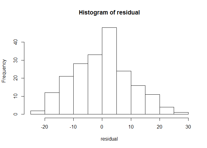
Plotting residuals
# Extract the residuals from the modelresidual<-resid(model_2)# Draw a histogram of the residualshist(residual)
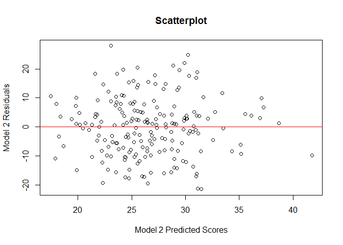
# Extract the predicted symptom scores from the modelpredicted<-fitted(model_2)# Plot the residuals against the predicted symptom scoresplot(residual~predicted,main='Scatterplot',ylab='Model 2 Residuals',xlab='Model 2 Predicted Scores')abline(lm(residual~predicted),col='red')